Can You Hear the Ball Bounce?
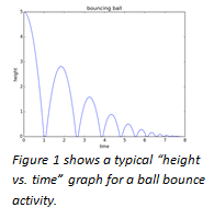 Most students instinctively know already that for each consecutive bounce, a ball will reach slightly less height than in the bounce before. They may have even explored the mathematical model that describes how the height decreases for a series of bounces, like the one shown in Figure 1. In physics classes, they might have explored the relationship between conservation of mechanical energy in the constant exchange between potential and kinetic energies and the diminishing rebound height.
In this ball bounce activity, we explore that relationship from a slightly different perspective. Can we develop a mathematical model that is based on the sound the ball makes on impact and the time interval between consecutive bounces? And can we then use our model to predict how long our ball would (theoretically) bounce?
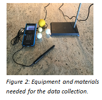 To get started, you’ll need the following equipment and materials (Figure 2):
- TI-Nspire™ CX or TI-Nspire™ CX II graphing calculator or a computer with TI-Nspire™ software
- TI-Nspire™ Lab Cradle
- Vernier microphone
- A handful of small balls (pingpong, golf, lacrosse — we’re not picky!)
Connect the microphone to one of the three analog ports on the TI-Nspire™ Lab Cradle. To avoid adding a page to an already open document, start a new document on the TI-Nspire™ CX family graphing calculator and open a page on the Vernier DataQuest™ App for TI-Nspire™ technology before attaching the TI-Nspire™ CX family graphing calculator to the TI-Nspire™ Lab Cradle.
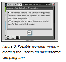 The correct setup of the TI-Nspire™ CX family graphing calculator is rather important for successful data collection. Set the mode to Time Based, and use a collection rate of about 750/sec with a duration of about 2.5–3 sec. Depending on the settings you choose, a warning window may pop up (Figure 3), alerting you to the fact that your sampling rate is not supported for the connected sensor or that it may exceed the available memory. This happens especially if the sampling rate and time are not evenly divisible. Simply click OK. Should the total number of samples exceed 2,500, the TI-Nspire™ CX family graphing calculator will adjust the settings automatically, or you can adjust the sampling rates if necessary.
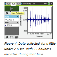 As can be seen in Figure 4, the sound is recorded in the form of air pressure variations in arbitrary units by the Vernier microphone. The sensor uses an electret microphone that has a frequency response covering essentially the range of the human ear to record the signal and then amplifies it through an op-amp circuit. For the data analysis, we zoomed in on two or three bounces at a time for more detail.
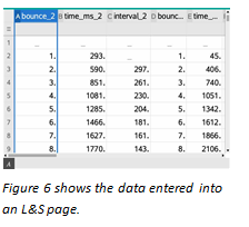
 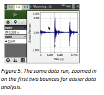 In Figure 5, the dotted line and the small circle show a time of .293 s, which corresponds to the first entry in cell B2 in the Lists & Spreadsheet (L&S) page (Figure 6). Record all those times, for as many bounces as possible, in the second column. Using these entries allows us to compute the difference in time between bounces and enter those in column C. Those time intervals in column C can then be plotted on a Data & Statistics page (Figure 7). Using the regression analysis function of the graphing calculator or the computer software, we can analyze our data and determine how well the mathematical model fits the experimental data. In this case, the regression model appears to fit the data well with little variance between predicted and actual values.
 Next, we took the data analysis one step further. We asked the question, what defines a good mathematical model? Let’s think about the question on how long the ball would bounce. We saw that, eventually, our ball came to rest. Theoretically, the ball would bounce an infinite number of times and the time between bounces would get shorter with each bounce. Is this where the mathematical model breaks down and doesn’t represent physical reality anymore? What would be the total time for an infinite number of bounces?
 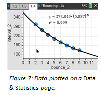 Instead of using the exponential regression to model the data, let’s use an infinite geometric series, in other words, a series with a constant ratio between successive terms. By adding a column to our L&S page like the one in Figure 6, we can verify that the ratio of successive time differences remains approximately constant and use that ratio in our geometric series.
Here a represents the initial time value, and b is the ratio of successive intervals.
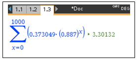
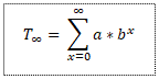 On the CAS model, you can store values for a and b, and then insert the summation template. Using the values from the function in Figure 7, for example, we get a total time of T=3,301 ms or 3.301 sec. In other words, our model shows that it would take a finite amount of time for an infinite number of bounces.
 These mathematical results can lead to some interesting discussions about how well the mathematical model describes the reality of the ball bounce.
On the numeric TI-Nspire™ CX or TI-Nspire™ CX II model, open a calculator page (or notes page with math template), insert the summation template and then the values for a and b, using a relatively high number for the upper limit of the sum (we picked 1,000).
 Hopefully, this activity, in which we explored a well-known relationship from a slightly different perspective, will inspire you to push even further. The time between bounces, in other words the time the ball spends in the air, can be thought of as the ball’s hang time. We can challenge students to consider variables they may be able to change to affect the hang time of the ball.
 What is the average hang time a human being might be able to achieve? Can you think of ways to measure it? What about top athletes? Did Michael Jordan really have such exceptional hang time?
Vernier DataQuest is a trademark of Vernier Software & Technology.
About the author: Karlheinz Haas (@karl0294) teaches AP® Physics, AP® Statistics and a STEM Lab class at The Pine School in Hobe Sound, Florida. Before coming to Florida, he taught science and mathematics in New Jersey and worked as an administrator in several school districts, in roles ranging from Math/Science Supervisor to Director of Curriculum and Assistant Superintendent. Haas is a National T³™ instructor, presenting regularly at Texas Instrument’s T³™ International Conference and at the annual NSTA STEM Forum & Expo. He sees the integration of technology as a great way to help students make connections between math and science.
Tagcloud
Archive
- 2026
- 2025
- 2024
- 2023
- 2022
-
2021
- January (1)
- February (2)
- March (5)
-
April (6)
- Top Tips for Tackling the SAT® with the TI-84 Plus CE
- Monday Night Calculus With Steve Kokoska and Tom Dick
- Which TI Calculator for the SAT® and Why?
- Top Tips From a Math Teacher for Taking the Online AP® Exam
- Celebrate National Robotics Week With Supervised Teardowns
- AP® Statistics: 6 Math Functions You Must Know for the TI-84 Plus
- May (1)
- June (3)
- July (2)
- August (5)
- September (2)
-
October (4)
- Transformation Graphing — the Families of Functions Modular Video Series to the Rescue!
- Top 3 Halloween-Themed Classroom Activities
- In Honor of National Chemistry Week, 5 “Organic” Ways to Incorporate TI Technology Into Chemistry Class
- 5 Spook-tacular Ways to Bring the Halloween “Spirits” Into Your Classroom
- November (4)
- December (1)
- 2020
- 2019
-
2018
- January (1)
- February (5)
- March (4)
- April (5)
- May (4)
- June (4)
- July (4)
- August (4)
- September (5)
- October (8)
-
November (8)
- Testing Tips: Using Calculators on Class Assessments
- Girls in STEM: A Personal Perspective
- 5 Teachers You Should Be Following on Instagram Right Now
- Meet TI Teacher of the Month: Katie England
- End-of-Marking Period Feedback Is a Two-Way Street
- #NCTMregionals Kansas City 2018 Recap
- Slope: It Shouldn’t Just Be a Formula
- Hit a high note exploring the math behind music
- December (5)
- 2017
- 2016
- 2015