Investigating Inverse Functions With the TI-84 Plus CE Graphing Calculator
Posted 06/09/2023 by Scott Knapp, Math Educator, T³™ Regional Instructor
A particular topic that really struck me is “inverse functions.” Why? Students often struggle with making connections between the definition of and various properties of inverse functions. In addition, students greatly benefit when function-related lessons include an emphasis on the multiple views of a function. TI technology to the rescue!
Let’s take a closer look at how TI technology, specifically the TI-84 Plus CE, can play an important role in supporting students to validate the meaning and properties of inverse functions. The great news is that TI has already done the work to provide teachers with resources to help effectively use technology to teach concepts like inverse functions. Be sure to access this “inverse functions” and other video tutorials for implementing the TI-84 Plus CE into math lessons involving inverse functions as well as links to videos for additional math topics.
Introducing inverse functions
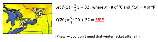
Suppose your family takes a road trip to visit Toronto for a long weekend. Upon arrival, a quick glance at a weather map is initially terrifying. You quickly remember that Canada uses ° Celsisus for its temperatures and there is a function you learned that converts from ° Celsisus to ° Fahrenheit. Find the corresponding temperature for Toronto in ° Fahrenheit.
Once students have made the conversion from the ℃ temperature to ℉, I challenge students to suppose the “inverse” role of someone visiting Chicago from Canada and to find the corresponding temperature in ℃ from a map of U.S. temperatures, in ℉, using f(x).
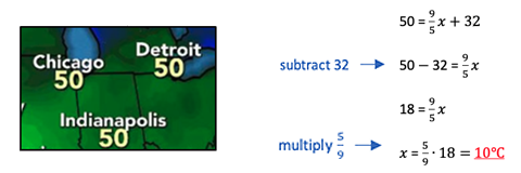
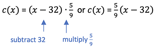
As students solve for the input of the function, in ℃, yielding 50℉, I encourage students to list the operations used in solving for the input (as shown above). This ultimately helps students construct the inverse function, c(x), where x = # of ℉ and c(x) = # of ℃:
Typically, when teaching math lessons, we teach skills first and then present applications. However, when teaching inverse functions, I prefer to start the lesson by introducing an application of inverse functions as a means of teaching the purpose and skill of finding inverse functions. This exercise establishes both the meaning of inverse functions and how to construct an inverse function … but we’re just getting started! Now it’s time to take a deeper dive into inverse functions by leveraging TI-84 Plus CE technology to validate the meaning and properties of inverse functions with an emphasis on the “three views” of functions.
The TI-84 Plus CE and the three views of a function
Function rule view
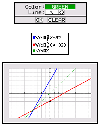
Type the functions f(x) and c(x) into a TI-84 Plus CE for Y1 and Y2, respectively. Then, from a calculator screen, compute the outputs of Y1 and Y2 as shown for students to confirm the inverse relationship. Because f(x) are c(x) inverse functions, f(a)=b implies c(b)=a.
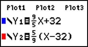
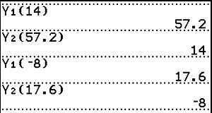
Table view
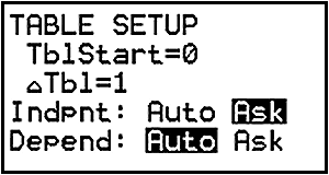
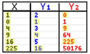
Construct a table to observe more examples of the numeric relationship between inverse functions. Set up the table by pressing [2nd] [window] to access the - . Select Ask so the table will be constructed by values entered for the independent variable.
Type the set of x-values shown below (in the first column) to calculate the outputs of Y1 and Y2, the two inverse functions. I like how the table view (see table 1) shows that the outputs of the two functions are different for a given input, but that using the output from one of the two inverse functions as the input into the other function, gives you the same original input into the first function (see highlighted values).
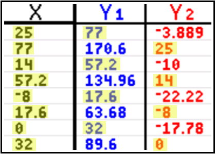
X = 25, 77 and Y1 and Y2 = 77, 25
X = 14, 57.2 and Y1 and Y2 = 57.2, 14
X = -8, 17.6 and Y1 and Y2 = 17.6, -8
X = 0, 32 and Y1 and Y2 = 32, 0
Graphing view
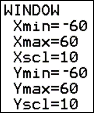
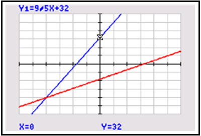
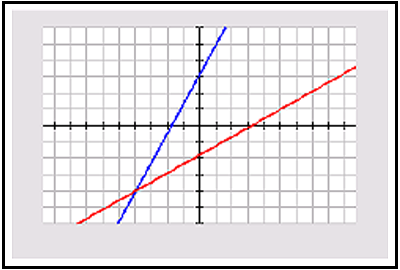
Press [window] and set up the graphing window as shown. This allows an appropriate domain and range for f(x), in Y1, and c(x), in Y2 to be viewed.
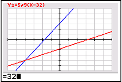
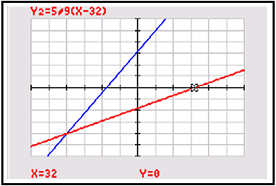
Press [graph] to graph the inverse functions entered in Y1 and Y2. Press [trace] and a flashing cursor will appear on the graph of Y1 (see screenshot 1 below). This represents the point (0, 32) on the graph of the function Y1 (keep in mind this means that 0℃ is equivalent to 32℉). Press [arrow down] to move to function Y2 and type 32 (see screenshot 2 below) using the keypad. Voila! The inverse relationship is now confirmed graphically.
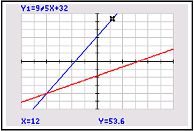
Try it again for another pair (or more!) of values!

Properties of inverse functions
Graphs of inverse functions
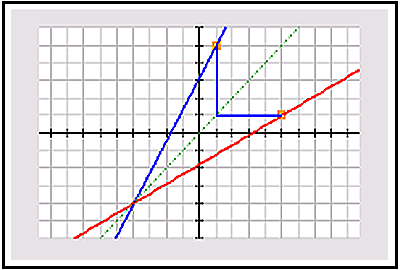
Not only is the TI-84 Plus CE a great tool for verifying functions are inverses using the various function views, but the TI-84 Plus CE also can be used to confirm properties of inverse functions. The first property involves the graphs of inverse functions. First, it would be helpful to view the two lines on a “square window.” Press [zoom] and ZSquare to have the viewing window update to be square. Then, look for patterns between the two graphs.
Many students observe the symmetry between the graphs of the two inverse functions, but given that the symmetry isn’t over the x- or y- axis (as many previous relationships involving symmetry have been), students sometimes struggle to locate the position for the line of symmetry. Usually, I ask a student volunteer to come to the emulator projection and “be” (with their arm) the line of symmetry. Then, I ask students if they can determine the equation of the line/arm. It sometimes takes a little prompting, but most classes determine the line is y=x, and we graph the line of symmetry as a dashed line for visual confirmation (screenshot 4 below).
This leads to a nice great discussion about why y=x makes sense. First, any points on either inverse function with the same x and y- values would not change when inverted. Second, it’s helpful to pick two corresponding points on the inverse functions and count their “path” to the line y=x (screenshot 5 below). For example, f(10)=50 is 40 units above the line y=x, while c(50)=10 is 40 units to the right of y=x. It might also be worth circling back to the equidistance theorem from geometry for even more support.
Compositions of inverse functions
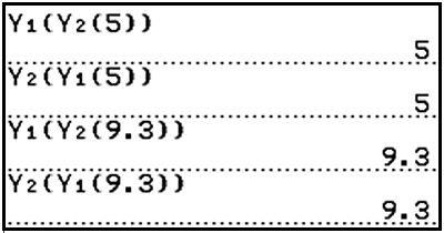
The TI-84 Plus CE makes investigating the composition property of inverse functions powerful and efficient. Have students calculate composition expressions involving both Y1(Y2(x)) and Y2(Y1(x)). I like to first have students use each function separately (see screenshot 6) and then as a full composition expression (see screenshot 7).
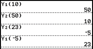

Students realize the pattern that Y1(Y2(x))=Y2(Y1(x)) are both equal to x no matter what x values are used. Ideally, this makes great sense because the compositions of inverse functions “undo” one another. (The context of the temperature functions definitely helps students understand the relationship better.) Students can then construct compositions for f(c(x)) and c(f(x)) that result in x.
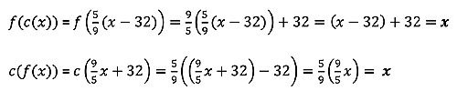
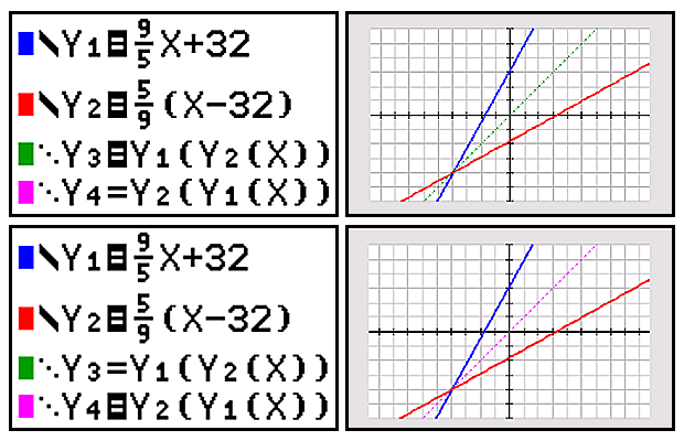
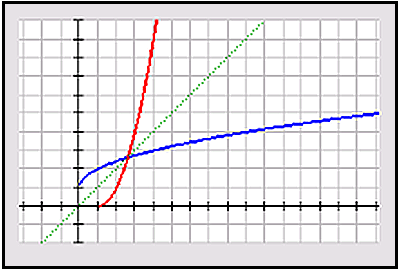
One final way to leverage the TI-84 Plus CE is to plot the compositions of the inverse functions, which end up graphing the line y=x when Y3=Y1(Y2(x)) and Y4=Y2(Y1(x)).
One final task
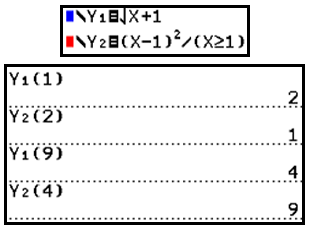
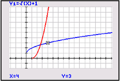
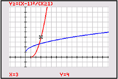
After students have observed the power of the TI-84 Plus CE, it’s worth giving them a chance to use the technology to observe the same relationships between a new pair of inverse functions. I personally like to use non-linear functions in this task.
Let a(x)=√x+1 and b(x)=(x-1)^2 for x≥1.
[Note: The domain restriction for b(x) is due to the range of a(x) being y≥1.]
If you are looking for more ideas on how to use the TI-84 Plus CE effectively in your classroom, visit this playlist to view other videos related to the TI-84 Plus CE.
About the author: Scott Knapp has been teaching math for 23 years and has served as a T³™ Regional Instructor for 12 years. He currently teaches at Glenbrook North High School in Northbrook, Illinois, a northern suburb of Chicago. Knapp is an advocate for using TI technology and regularly presents at conferences, workshops and webinars, demonstrating how TI technology can be effectively used by students to explore and learn mathematics. Follow Knapp on Twitter @scottknapp.