How Else Can We Show This?
What I love about using calculator technology in my teaching is the “Power of Visualization” and the opportunity to examine math through different lenses. The multiple representations available on Texas Instruments (TI) graphing calculators — numeric, algebraic, graphical, geometric, statistical — allow me to push my students to approach problems in more than one “right way.” By connecting these environments and making student thinking visible when we dig into a mathematical situation, we support students in productive struggle and deepen their understanding.*
Read on for two scenarios in which my students and I pursue multiple pathways to show and make sense of the mathematics at hand.
1. Riding the Curves and Turning the Tables
When studying quadratic and polynomial functions, I begin by having students tell me everything they see on a graph. They mention things like y-intercepts, x-intercepts, high points and low points. We use TRACE and the commands in the CALC menu to find these points if they aren’t apparent by visual inspection.
I then ask students if they can find a place in the equation of a quadratic function that reveals each of these graph features. Standard form clearly shows the y-intercept, factored form gives the x-intercepts (if any), and vertex form indicates the high or low point. We use the “tracer ball” graphing style on the TI-84 Plus graphing calculator family to connect each of these equations, confirm whether they are equivalent, and to be sure that we factored or expanded or completed the square correctly. This video shows the process for Y = x2 – 5x + 4.
;
Once we have found the important points in the function’s graph and in the equation, I ask my students, “What exactly is going on at these points?” and have them investigate using TRACE and the Table. The ZoomDecimal window provides a “friendly” trace increment of 0.1, and students can start to see what happens at the intercepts and relative extrema of the function.
The GRAPH-TABLE split screen enhances the exploration, allowing students to observe what is happening numerically at each of the key points. At the x-intercepts (zeros) of the function, the Y-values change sign. At the y-intercept, the X-value is 0. At a relative maximum, the Y-values increase then decrease; at a minimum, the opposite is true. In order to make this numerical behavior apparent, use a smaller Table increment DTBL to “zoom in” on the table.
This video shows the process for Y = x3 – 2x2 – x + 3. For this function, the relative maximum is close to the y-intercept, so the “zooming in” process helps us distinguish between them. Students explain their thinking in words and confirm their understanding with the calculator. This also lays the groundwork for some concepts in calculus.
;
2. Absolute Certainty
When most students first learn of absolute value, it is an easy idea to grasp — it “turns numbers positive” if they aren’t already. Unfortunately, that procedural rule isn’t robust enough to take students through to graphing absolute value functions and solving absolute value equations and inequalities, some of the difficult topics they might encounter in algebra class.
With my students, I have expanded our view of absolute value to mean “the distance on the number line to zero.” For a question such as “Solve |x – 2|= 3”, we focus on the 3, so we find the places on the number line that are three units away from zero, namely 3 and -3. This “distance” context supports the procedure that is typically taught, to solve by creating two equations: x – 2 = 3 or x – 2 = -3.
But how else can we show this? By graphing the absolute value function Y1 = |x – 2| along with Y2 = 3, we can find the points of intersection that are solutions to the original equation. Further, we can draw in the vertical line through the vertex, and the distance from that line to the points of intersection is three units.
One more approach to this equation is to recognize that solving |x – 2|= 3 is equivalent to solving |x – 2|– 3 = 0. Students have studied transformations on parent functions and the translations that change Y = |x| into Y = |x – h|+ k. We enter Y3 = |x – 2|– 3 and notice that the zeros of this function are the same X-values of the points of intersection we found earlier.
;
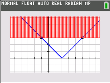
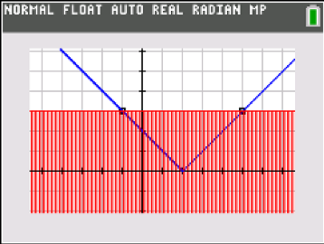
The graphical environment is also helpful with absolute value inequalities. Choose the “shade above” graphing style to solve |x – 2|> 3 and the “shade below” style to solve |x – 2|< 3. These visuals help students make sense of algebraic solution methods that create compound inequalities to solve; the graphs are grounded in mathematical meaning and are a big improvement over rote memorization of the trick “great-OR / less-thAND”. />
*Connecting mathematical representations and supporting productive struggle are two of the high-leverage mathematical teaching practices discussed in NCTM’s “Principles to Actions: Ensuring Mathematical Success for All” (2014).
About the author: Karen Campe is a T3™ National Instructor with 15 years’ experience teaching secondary math and pre-service teachers. She is passionate about using all types of technology to enhance student understanding in mathematics and has provided technology professional development at conferences, workshops and webinars since 1998. Karen blogs at karendcampe.wordpress.com. Follow her on Twitter @KarenCampe.
Tagcloud
Archive
- 2026
- 2025
- 2024
- 2023
- 2022
-
2021
- January (1)
- February (2)
- March (5)
-
April (6)
- Top Tips for Tackling the SAT® with the TI-84 Plus CE
- Monday Night Calculus With Steve Kokoska and Tom Dick
- Which TI Calculator for the SAT® and Why?
- Top Tips From a Math Teacher for Taking the Online AP® Exam
- Celebrate National Robotics Week With Supervised Teardowns
- AP® Statistics: 6 Math Functions You Must Know for the TI-84 Plus
- May (1)
- June (3)
- July (2)
- August (5)
- September (2)
-
October (4)
- Transformation Graphing — the Families of Functions Modular Video Series to the Rescue!
- Top 3 Halloween-Themed Classroom Activities
- In Honor of National Chemistry Week, 5 “Organic” Ways to Incorporate TI Technology Into Chemistry Class
- 5 Spook-tacular Ways to Bring the Halloween “Spirits” Into Your Classroom
- November (4)
- December (1)
- 2020
- 2019
-
2018
- January (1)
- February (5)
- March (4)
- April (5)
- May (4)
- June (4)
- July (4)
- August (4)
- September (5)
- October (8)
-
November (8)
- Testing Tips: Using Calculators on Class Assessments
- Girls in STEM: A Personal Perspective
- 5 Teachers You Should Be Following on Instagram Right Now
- Meet TI Teacher of the Month: Katie England
- End-of-Marking Period Feedback Is a Two-Way Street
- #NCTMregionals Kansas City 2018 Recap
- Slope: It Shouldn’t Just Be a Formula
- Hit a high note exploring the math behind music
- December (5)
- 2017
- 2016
- 2015