TI-89 Titanium Graphing Calculator Lesson
Module 16: The Fundamental Theorem of Calculus
Introduction | Lesson 1 | Lesson 2 | Lesson 3 | Self-Test
Lesson 16.2: Area Functions, A Visual Approach
This lesson develops area functions using a visual approach by exploring the values of the areas under a curve when the right-hand endpoint changes. The visualization is displayed by graphing a definite integral in which the right end point is variable.
If the curve and the left-hand endpoint are given, an area function can be found for a right-hand endpoint that varies. It's necessary to distinguish between the independent variables for the curve function and for the area function. If x is used to denote the variable right-hand endpoint of the region, a second variable, t, should be used in the description of the curve function.
Letting x represent the right-hand endpoint, the area under the curve
![]() and above the t-axis between t = 1 and t = x can be found by evaluating the definite integral
and above the t-axis between t = 1 and t = x can be found by evaluating the definite integral
![]() .
.
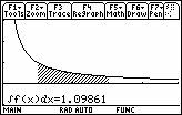
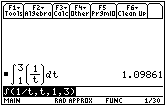
For example, if x = 3 the area under the curve between x = 1 and x = 3 is about 1.09861, as illustrated and evaluated in the screens below.
16.2.1 Put your calculator in Approximate mode or just press
![]()
![]() to get the decimal values, and use the definite integral key to find the areas under
to get the decimal values, and use the definite integral key to find the areas under
![]() between 1 and the following values of x. Record your results in the table.
between 1 and the following values of x. Record your results in the table.
| x | 1.0 | 1.5 | 2.0 | 2.5 | 3.0 | 3.5 | 4.0 |
| Area |
Click here for the answer.
16.2.2 Make a scatter plot of your results and find the logarithmic regression equation that best fits the data. Graph this equation together with the scatter plot.
Click on scatter plot or regression equation to review the associated keystrokes.
Click here for the answer.
Based on this data, it appears that the area function, A(x), may be ln x.
Graphing Integrals
Graph
![]() together with the scatter plot.
together with the scatter plot.
- Disable or delete the regression equation in the Y=Editor
-
Set
 and use the window [0.01, 4.5] x [-5, 2]
- Graph the equation y1
The graph will be slow to appear because the calculator has to compute a new definite integral for each point it plots. You should see the area function
![]() develop point by point.
develop point by point.
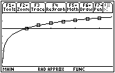
Notice that the graph of A(x) appears to be the same as the graph of the ln x, the regression equation we found above.
16.2.3 Based on these graphs, predict the values of
![]() .
.
Click here for the answer.
16.2.4 Describe how the Fundamental theorem applies.
Click here to see the answer.
Visualizing
![]()
Suppose that you don't know a formula for the curve function but you have its graph. You can determine the shape of the area function by analyzing the graph of the curve.
Below is the graph of
![]() on the interval from 1 to x that was developed earlier.
on the interval from 1 to x that was developed earlier.
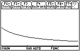
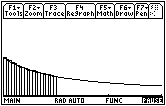
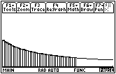
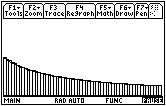
Visualize the area under the graph of f being filled with thin rectangular sticks where the height of each stick is the y-value of the curve function. Each successive rectangular stick is shorter than the prior one. The Riemann sum is growing more slowly with each step as you move to the right because the area of each successive rectangle is less than the one before, as shown below.
Using the Fundamental Theorem
The Fundamental Theorem states that the derivative of the area function is the curve function. That means that the curve function values correspond to slopes of tangent lines of the area function.
Some of the characteristics of the area function that can be determined from the graph of the curve function are listed below.
- A curve function's y-value at x is the slope of the tangent line of the area function at that x-value.
- When the curve function is decreasing, the area function's slopes are decreasing and its graph is concave downward.
- When the curve function is increasing, the area function's slopes are increasing and its graph is concave upward.
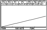
16.2.5 Examine the graph of f(x) between x = 0 and x = 4 shown below. Approximate the graph of the corresponding area function on the interval from 0 to 4.
Click here for the answer.
