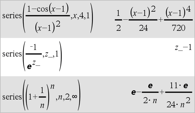
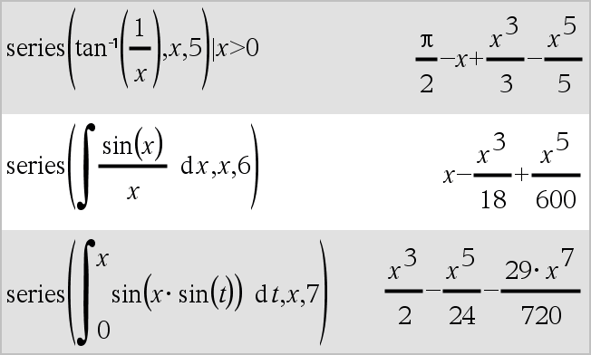
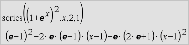
You are here: TI‑Nspire™ CX CAS Reference Guide > Alphabetical Listing > S

S

sec()

sec(Expr1) expression

sec(List1) list

Returns the secant of Expr1 or returns a list containing the secants of all elements in List1.

Note: The argument is interpreted as a degree, gradian or radian angle, according to the current angle mode setting. You can use °G, or r to override the angle mode temporarily.

In Degree angle mode:

sec¹()

sec¹(Expr1) expression

sec¹(List1) list

Returns the angle whose secant is Expr1 or returns a list containing the inverse secants of each element of List1.

Note: The result is returned as a degree, gradian, or radian angle, according to the current angle mode setting.

Note: You can insert this function from the keyboard by typing arcsec(...).

In Degree angle mode:


In Gradian angle mode:


In Radian angle mode:

sech()

sech(Expr1) expression

sech(List1) list

Returns the hyperbolic secant of Expr1 or returns a list containing the hyperbolic secants of the List1 elements.

sech¹()

sech¹(Expr1) expression

sech¹(List1) list

Returns the inverse hyperbolic secant of Expr1 or returns a list containing the inverse hyperbolic secants of each element of List1.

Note: You can insert this function from the keyboard by typing arcsech(...).

In Radian angle and Rectangular complex mode:

Send 

Send exprOrString1 [, exprOrString2] ...

Programming command: Sends one or more TI‑Innovator™ Hub commands to a connected hub.

exprOrString must be a valid TI‑Innovator™ Hub Command. Typically, exprOrString contains a "SET ..." command to control a device or a "READ ..." command to request data.

The arguments are sent to the hub in succession.

Note: You can use the Send command within a user-defined program but not within a function.

Note: See also Get (here), GetStr (here), and eval() (here).

Example: Turn on the blue element of the built-in RGB LED for 0.5 seconds.

Example: Request the current value of the hub's built-in light-level sensor. A Get command retrieves the value and assigns it to variable lightval.

Example: Send a calculated frequency to the hub's built-in speaker. Use special variable iostr.SendAns to show the hub command with the expression evaluated.

seq()

seq(Expr, Var, Low, High[, Step]) list

Increments Var from Low through High by an increment of Step, evaluates Expr, and returns the results as a list. The original contents of Var are still there after seq() is completed.

The default value for Step = 1.

Note: To force an approximate result,

Handheld: Press / ·.
Windows®:
Press Ctrl+Enter.
Macintosh®:
Press +Enter.
iPad®:
Hold enter, and select .

seqGen()

seqGen(Expr, Var, depVar, {Var0, VarMax}[, ListOfInitTerms
    [, VarStep[, CeilingValue]]]) list

Generates a list of terms for sequence depVar(Var)=Expr as follows: Increments independent variable Var from Var0 through VarMax by VarStep, evaluates depVar(Var) for corresponding values of Var using the Expr formula and ListOfInitTerms, and returns the results as a list.

seqGen(ListOrSystemOfExpr, Var, ListOfDepVars, {Var0, VarMax}    [
, MatrixOfInitTerms[, VarStep[, CeilingValue]]]) matrix

Generates a matrix of terms for a system (or list) of sequences ListOfDepVars(Var)=ListOrSystemOfExpr as follows: Increments independent variable Var from Var0 through VarMax by VarStep, evaluates ListOfDepVars(Var) for corresponding values of Var using ListOrSystemOfExpr formula and MatrixOfInitTerms, and returns the results as a matrix.

The original contents of Var are unchanged after seqGen() is completed.

The default value for VarStep = 1.

Generate the first 5 terms of the sequence u(n) = u(n-1)2/2, with u(1)=2 and VarStep=1.


Example in which Var0=2:


Example in which initial term is symbolic:


System of two sequences:

Note: The Void (_) in the initial term matrix above is used to indicate that the initial term for u1(n) is calculated using the explicit sequence formula u1(n)=1/n.

seqn()

seqn(Expr(u, n[, ListOfInitTerms[, nMax[, CeilingValue]]]) list

Generates a list of terms for a sequence u(n)=Expr(u, n) as follows: Increments n from 1 through nMax by 1, evaluates u(n) for corresponding values of n using the Expr(u, n) formula and ListOfInitTerms, and returns the results as a list.

seqn(Expr(n[, nMax[, CeilingValue]]) list

Generates a list of terms for a non-recursive sequence u(n)=Expr(n) as follows: Increments n from 1 through nMax by 1, evaluates u(n) for corresponding values of n using the Expr(n) formula, and returns the results as a list.

If nMax is missing, nMax is set to 2500

If nMax=0, nMax is set to 2500

Note: seqn() calls seqGen( ) with n0=1 and nstep =1

Generate the first 6 terms of the sequence u(n) = u(n-1)/2, with u(1)=2.

series()

series(Expr1, Var, Order[, Point]) expression

series(Expr1, Var, Order[, Point]) | Var>Point expression

series(Expr1, Var, Order[, Point]) | Var<Point expression


Returns a generalized truncated power series representation of Expr1 expanded about Point through degree Order. Order can be any rational number. The resulting powers of (Var Point) can include negative and/or fractional exponents. The coefficients of these powers can include logarithms of (Var  Point) and other functions of Var that are dominated by all powers of (Var Point) having the same exponent sign.

Point defaults to 0. Point can be or , in which cases the expansion is through degree Order in 1/(Var Point).

series(...) returns “series(...)” if it is unable to determine such a representation, such as for essential singularities such as sin(1/z) at z=0, e1/z at z=0, or ez at z = or .

If the series or one of its derivatives has a jump discontinuity at Point, the result is likely to contain sub-expressions of the form sign(…) or abs(…) for a real expansion variable or (-1)floor(…angle(…)…) for a complex expansion variable, which is one ending with “_”. If you intend to use the series only for values on one side of Point, then append the appropriate one of “| Var > Point”, “| Var < Point”, “| “Var Point”, or “Var Point” to obtain a simpler result.

series() can provide symbolic approximations to indefinite integrals and definite integrals for which symbolic solutions otherwise can't be obtained.

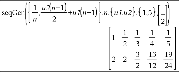
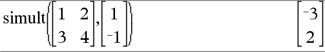
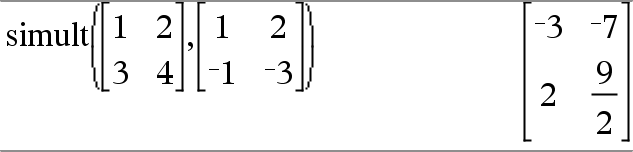
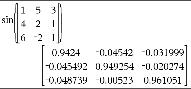
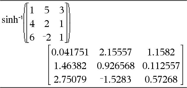
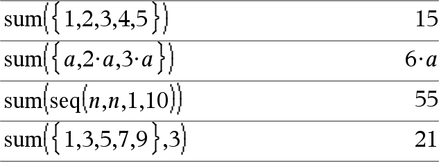
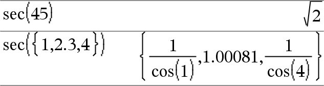
series() distributes over 1st-argument lists and matrices.

series() is a generalized version of taylor().

As illustrated by the last example to the right, the display routines downstream of the result produced by series(...) might rearrange terms so that the dominant term is not the leftmost one.

Note: See also dominantTerm(), here.

setMode()

setMode(modeNameInteger, settingInteger) integer
setMode(list) integer list

Valid only within a function or program.

setMode(modeNameInteger, settingInteger) temporarily sets mode modeNameInteger to the new setting settingInteger, and returns an integer corresponding to the original setting of that mode. The change is limited to the duration of the program/function’s execution.

modeNameInteger specifies which mode you want to set. It must be one of the mode integers from the table below.

settingInteger specifies the new setting for the mode. It must be one of the setting integers listed below for the specific mode you are setting.

setMode(list) lets you change multiple settings. list contains pairs of mode integers and setting integers. setMode(list) returns a similar list whose integer pairs represent the original modes and settings.

If you have saved all mode settings with getMode(0)var, you can use setMode(var) to restore those settings until the function or program exits. See getMode(), here.

Note: The current mode settings are passed to called subroutines. If any subroutine changes a mode setting, the mode change will be lost when control returns to the calling routine.

Note for entering the example: For instructions on entering multi-line program and function definitions, refer to the Calculator section of your product guidebook.

Display approximate value of π using the default setting for Display Digits, and then display π with a setting of Fix2. Check to see that the default is restored after the program executes.

Mode
Name

Mode
Integer


Setting Integers

Display Digits

1

1=Float, 2=Float1, 3=Float2, 4=Float3, 5=Float4, 6=Float5, 7=Float6, 8=Float7, 9=Float8, 10=Float9, 11=Float10, 12=Float11, 13=Float12, 14=Fix0, 15=Fix1, 16=Fix2, 17=Fix3, 18=Fix4, 19=Fix5, 20=Fix6, 21=Fix7, 22=Fix8, 23=Fix9, 24=Fix10, 25=Fix11, 26=Fix12

Angle

2

1=Radian, 2=Degree, 3=Gradian

Exponential Format

3

1=Normal, 2=Scientific, 3=Engineering

Real or Complex

4

1=Real, 2=Rectangular, 3=Polar

Auto or Approx.

5

1=Auto, 2=Approximate, 3=Exact

Vector Format

6

1=Rectangular, 2=Cylindrical, 3=Spherical

Base

7

1=Decimal, 2=Hex, 3=Binary

Unit system

8

1=SI, 2=Eng/US

shift()

shift(Integer1[,#ofShifts]) integer

Shifts the bits in a binary integer. You can enter Integer1 in any number base; it is converted automatically to a signed, 64-bit binary form. If the magnitude of Integer1 is too large for this form, a symmetric modulo operation brings it within the range. For more information, see Base2,  here.

If #ofShifts is positive, the shift is to the left. If #ofShifts is negative, the shift is to the right. The default is 1 (shift right one bit).

In a right shift, the rightmost bit is dropped and 0 or 1 is inserted to match the leftmost bit. In a left shift, the leftmost bit is dropped and 0 is inserted as the rightmost bit.

For example, in a right shift:

Each bit shifts right.

0b0000000000000111101011000011010

Inserts 0 if leftmost bit is 0,
or 1 if leftmost bit is 1.

produces:

0b00000000000000111101011000011010

The result is displayed according to the Base mode. Leading zeros are not shown.

In Bin base mode:


In Hex base mode:

Important: To enter a binary or hexadecimal number, always use the 0b or 0h prefix (zero, not the letter O).

shift(List1[,#ofShifts]) list

Returns a copy of List1 shifted right or left by #ofShifts elements. Does not alter List1.

If #ofShifts is positive, the shift is to the left. If #ofShifts is negative, the shift is to the right. The default is 1 (shift right one element).

Elements introduced at the beginning or end of list by the shift are set to the symbol “undef”.

In Dec base mode:

shift(String1[,#ofShifts]) string

Returns a copy of String1 shifted right or left by #ofShifts characters. Does not alter String1.

If #ofShifts is positive, the shift is to the left. If #ofShifts is negative, the shift is to the right. The default is 1 (shift right one character).

Characters introduced at the beginning or end of string by the shift are set to a space.

sign()

sign(Expr1) expression

sign(List1) list
sign(Matrix1) matrix

For real and complex Expr1, returns Expr1/abs(Expr1) when Expr1 0.

Returns 1 if Expr1 is positive. Returns 1 if Expr1is negative.

sign(0) represents the unit circle in the complex domain.

For a list or matrix, returns the signs of all the elements.


If complex format mode is Real:

simult()

simult(coeffMatrix, constVector[, Tol]) matrix

Returns a column vector that contains the solutions to a system of linear equations.

Note: See also linSolve(), here.

coeffMatrix must be a square matrix that contains the coefficients of the equations.

constVector must have the same number of rows (same dimension) as coeffMatrix and contain the constants.

Optionally, any matrix element is treated as zero if its absolute value is less than Tol. This tolerance is used only if the matrix has floating-point entries and does not contain any symbolic variables that have not been assigned a value. Otherwise, Tol is ignored.

If you set the Auto or Approximate mode to Approximate, computations are done using floating-point arithmetic.
If Tol is omitted or not used, the default tolerance is calculated as:
5E14 max(dim(coeffMatrix)) rowNorm(coeffMatrix)

Solve for x and y:
x + 2y = 1
3x + 4y = 1

The solution is x=3 and y=2.


Solve:
ax + by = 1
cx + dy = 2

simult(coeffMatrix, constMatrix[, Tol]) matrix

Solves multiple systems of linear equations, where each system has the same equation coefficients but different constants.

Each column in constMatrix must contain the constants for a system of equations. Each column in the resulting matrix contains the solution for the corresponding system.

Solve:
  x + 2y = 1
3x + 4y = 1

  x + 2y = 2
3x + 4y = 3

For the first system, x=3 and y=2. For the second system, x=7 and y=9/2.

sin

Exprsin

Note: You can insert this operator from the computer keyboard by typing @>sin.

Represents Expr in terms of sine. This is a display conversion operator. It can be used only at the end of the entry line.

sin reduces all powers of
    cos(...) modulo 1sin(...)^2
so that any remaining powers of sin(...) have exponents in the range (0, 2). Thus, the result will be free of cos(...) if and only if cos(...) occurs in the given expression only to even powers.

Note: This conversion operator is not supported in Degree or Gradian Angle modes. Before using it, make sure that the Angle mode is set to Radians and that Expr does not contain explicit references to degree or gradian angles.


sin()

sin(Expr1) expression

sin(List1) list

sin(Expr1) returns the sine of the argument as an expression.

sin(List1) returns a list of the sines of all elements in List1.

Note: The argument is interpreted as a degree, gradian or radian angle, according to the current angle mode. You can use °, g, or r to override the angle mode setting temporarily.

In Degree angle mode:


In Gradian angle mode:


In Radian angle mode:

sin(squareMatrix1) squareMatrix

Returns the matrix sine of squareMatrix1. This is not the same as calculating the sine of each element. For information about the calculation method, refer to cos().

squareMatrix1 must be diagonalizable. The result always contains floating-point numbers.

In Radian angle mode:

sin¹()

sin¹(Expr1) expression

sin¹(List1) list

sin¹(Expr1) returns the angle whose sine is Expr1 as an expression.

sin¹(List1) returns a list of the inverse sines of each element of List1.

Note: The result is returned as a degree, gradian or radian angle, according to the current angle mode setting.

Note: You can insert this function from the keyboard by typing arcsin(...).

In Degree angle mode:


In Gradian angle mode:


In Radian angle mode:

sin¹(squareMatrix1) squareMatrix

Returns the matrix inverse sine of squareMatrix1. This is not the same as calculating the inverse sine of each element. For information about the calculation method, refer to cos().

squareMatrix1 must be diagonalizable. The result always contains floating-point numbers.

In Radian angle mode and Rectangular complex format mode:

sinh()

sinh(Expr1) expression

sinh(List1) list

sinh (Expr1) returns the hyperbolic sine of the argument as an expression.

sinh (List1) returns a list of the hyperbolic sines of each element of List1.

sinh(squareMatrix1) squareMatrix

Returns the matrix hyperbolic sine of squareMatrix1. This is not the same as calculating the hyperbolic sine of each element. For information about the calculation method, refer to cos().

squareMatrix1 must be diagonalizable. The result always contains floating-point numbers.

In Radian angle mode:

sinh¹()

sinh¹(Expr1) expression

sinh¹(List1) list

sinh¹(Expr1) returns the inverse hyperbolic sine of the argument as an expression.

sinh¹(List1) returns a list of the inverse hyperbolic sines of each element of List1.

Note: You can insert this function from the keyboard by typing arcsinh(...).

sinh¹(squareMatrix1) squareMatrix

Returns the matrix inverse hyperbolic sine of squareMatrix1. This is not the same as calculating the inverse hyperbolic sine of each element. For information about the calculation method, refer to cos().

squareMatrix1 must be diagonalizable. The result always contains floating-point numbers.

In Radian angle mode:

SinReg

SinReg X, Y[, [Iterations],[Period][, Category, Include]]

Computes the sinusoidal regression on lists X and Y. A summary of results is stored in the stat.results variable. (See here.)

All the lists must have equal dimension except for Include.

X and Y are lists of independent and dependent variables.

Iterations is a value that specifies the maximum number of times (1 through 16) a solution will be attempted. If omitted, 8 is used. Typically, larger values result in better accuracy but longer execution times, and vice versa.

Period specifies an estimated period. If omitted, the difference between values in X should be equal and in sequential order. If you specify Period, the differences between x values can be unequal.

Category is a list of category codes for the corresponding X and Y data.

Include is a list of one or more of the category codes. Only those data items whose category code is included in this list are included in the calculation.

The output of SinReg is always in radians, regardless of the angle mode setting.

For information on the effect of empty elements in a list, see “Empty (Void) Elements,” here.


Output variable

Description

stat.RegEqn

Regression Equation: asin(bx+c)+d

stat.a, stat.b, stat.c, stat.d

Regression coefficients

stat.Resid

Residuals from the regression

stat.XReg

List of data points in the modified X List actually used in the regression based on restrictions of Freq, Category List, and Include Categories

stat.YReg

List of data points in the modified Y List actually used in the regression based on restrictions of Freq, Category List, and Include Categories

stat.FreqReg

List of frequencies corresponding to stat.XReg and stat.YReg

solve()

solve(Equation, Var) Boolean expression
solve(Equation, Var=Guess) Boolean expression
solve(Inequality, Var) Boolean expression

Returns candidate real solutions of an equation or an inequality for Var. The goal is to return candidates for all solutions. However, there might be equations or inequalities for which the number of solutions is infinite.

Solution candidates might not be real finite solutions for some combinations of values for undefined variables.

For the Auto setting of the Auto or Approximate mode, the goal is to produce exact solutions when they are concise, and supplemented by iterative searches with approximate arithmetic when exact solutions are impractical.

Due to default cancellation of the greatest common divisor from the numerator and denominator of ratios, solutions might be solutions only in the limit from one or both sides.

For inequalities of types , , <, or >, explicit solutions are unlikely unless the inequality is linear and contains only Var.

For the Exact mode, portions that cannot be solved are returned as an implicit equation or inequality.

Use the constraint (“|”) operator to restrict the solution interval and/or other variables that occur in the equation or inequality. When you find a solution in one interval, you can use the inequality operators to exclude that interval from subsequent searches.

In Radian angle mode:

false is returned when no real solutions are found. true is returned if solve() can determine that any finite real value of Var satisfies the equation or inequality.

Since solve() always returns a Boolean result, you can use “and,” “or,” and “not” to combine results from solve() with each other or with other Boolean expressions.

Solutions might contain a unique new undefined constant of the form nj with j being an integer in the interval 1–255. Such variables designate an arbitrary integer.

In Radian angle mode:

In Real mode, fractional powers having odd denominators denote only the real branch. Otherwise, multiple branched expressions such as fractional powers, logarithms, and inverse trigonometric functions denote only the principal branch. Consequently, solve() produces only solutions corresponding to that one real or principal branch.

Note: See also cSolve(), cZeros(), nSolve(), and zeros().

solve(Eqn1 and Eqn2[and ], VarOrGuess1, VarOrGuess2[, ])  Boolean expression

solve(SystemOfEqns, VarOrGuess1, VarOrGuess2[, ])  Boolean expression

solve({Eqn1, Eqn2 [,...]} {VarOrGuess1,VarOrGuess2 [, … ]})  Boolean expression

Returns candidate real solutions to the simultaneous algebraic equations, where each VarOrGuess specifies a variable that you want to solve for.

You can separate the equations with the and operator, or you can enter a SystemOfEqns using a template from the Catalog. The number of VarOrGuess arguments must match the number of equations. Optionally, you can specify an initial guess for a variable. Each VarOrGuess must have the form:

variable
– or –
variable = real or non-real number

For example, x is valid and so is x=3.

If all of the equations are polynomials and if you do NOT specify any initial guesses, solve() uses the lexical Gröbner/Buchberger elimination method to attempt to determine all real solutions.

For example, suppose you have a circle of radius r at the origin and another circle of radius r centered where the first circle crosses the positive x-axis. Use solve() to find the intersections.

As illustrated by r in the example to the right, simultaneous polynomial equations can have extra variables that have no values, but represent given numeric values that could be substituted later.

You can also (or instead) include solution variables that do not appear in the equations. For example, you can include z as a solution variable to extend the previous example to two parallel intersecting cylinders of radius r.

The cylinder solutions illustrate how families of solutions might contain arbitrary constants of the form ck, where k is an integer suffix from 1 through 255.

For polynomial systems, computation time or memory exhaustion may depend strongly on the order in which you list solution variables. If your initial choice exhausts memory or your patience, try rearranging the variables in the equations and/or varOrGuess list.

To see the entire result,
press 5 and then use 7 and 8 to move the cursor.

If you do not include any guesses and if any equation is non-polynomial in any variable but all equations are linear in the solution variables, solve() uses Gaussian elimination to attempt to determine all real solutions.

If a system is neither polynomial in all of its variables nor linear in its solution variables, solve() determines at most one solution using an approximate iterative method. To do so, the number of solution variables must equal the number of equations, and all other variables in the equations must simplify to numbers.

To see the entire result,
press 5 and then use 7 and 8 to move the cursor.

Each solution variable starts at its guessed value if there is one; otherwise, it starts at 0.0.

Use guesses to seek additional solutions one by one. For convergence, a guess may have to be rather close to a solution.


SortA

SortA List1[, List2] [, List3]...
SortA Vector1[, Vector2] [, Vector3]...

Sorts the elements of the first argument in ascending order.

If you include additional arguments, sorts the elements of each so that their new positions match the new positions of the elements in the first argument.

All arguments must be names of lists or vectors. All arguments must have equal dimensions.

Empty (void) elements within the first argument move to the bottom. For more information on empty elements, see here.


SortD

SortD List1[, List2][, List3]...
SortD Vector1[,Vector2][,Vector3]...

Identical to SortA, except SortD sorts the elements in descending order.

Empty (void) elements within the first argument move to the bottom. For more information on empty elements, see here.

Sphere

VectorSphere

Note: You can insert this operator from the computer keyboard by typing @>Sphere.

Displays the row or column vector in spherical form [ρθφ].

Vector must be of dimension 3 and can be either a row or a column vector.

Note: Sphere is a display-format instruction, not a conversion function. You can use it only at the end of an entry line.

Note: To force an approximate result,

Handheld: Press / ·.
Windows®:
Press Ctrl+Enter.
Macintosh®:
Press +Enter.
iPad®:
Hold enter, and select .


Press ·

sqrt()

sqrt(Expr1) expression

sqrt(List1) list

Returns the square root of the argument.

For a list, returns the square roots of all the elements in List1.

Note: See also Square root template, here.

stat.results

stat.results

Displays results from a statistics calculation.

The results are displayed as a set of name-value pairs. The specific names shown are dependent on the most recently evaluated statistics function or command.

You can copy a name or value and paste it into other locations.


Note: Avoid defining variables that use the same names as those used for statistical analysis. In some cases, an error condition could occur. Variable names used for statistical analysis are listed in the table below.

stat.a

stat.AdjR²

stat.b

stat.b0

stat.b1

stat.b2

stat.b3

stat.b4

stat.b5

stat.b6

stat.b7

stat.b8

stat.b9

stat.b10

stat.bList

stat.χ²

stat.c

stat.CLower

stat.CLowerList

stat.CompList

stat.CompMatrix

stat.CookDist

stat.CUpper

stat.CUpperList

stat.d

stat.dfDenom

stat.dfBlock

stat.dfCol

stat.dfError

stat.dfInteract

stat.dfReg

stat.dfNumer

stat.dfRow

stat.DW

stat.e

stat.ExpMatrix

stat.F

stat.FBlock

stat.Fcol

stat.FInteract

stat.FreqReg

stat.Frow

stat.Leverage

stat.LowerPred

stat.LowerVal

stat.m

stat.MaxX

stat.MaxY

stat.ME

stat.MedianX

stat.MedianY

stat.MEPred

stat.MinX

stat.MinY

stat.MS

stat.MSBlock

stat.MSCol

stat.MSError

stat.MSInteract

stat.MSReg

stat.MSRow

stat.n

Stat.Ç

stat.Ç1

stat.Ç2

stat.ÇDiff

stat.PList

stat.PVal

stat.PValBlock

stat.PValCol

stat.PValInteract

stat.PValRow

stat.Q1X

stat.Q1Y

stat.Q3X

stat.Q3Y

stat.r

stat.r²

stat.RegEqn

stat.Resid

stat.ResidTrans

stat.σx

stat.σy

stat.σx1

stat.σx2

stat.Σx

stat.Σx²

stat.Σxy

stat.Σy

stat.Σy²

stat.s

stat.SE

stat.SEList

stat.SEPred

stat.sResid

stat.SEslope

stat.sp

stat.SS

stat.SSBlock

stat.SSCol

stat.SSX

stat.SSY

stat.SSError

stat.SSInteract

stat.SSReg

stat.SSRow

stat.tList

stat.UpperPred

stat.UpperVal

stat.v

stat.v1

stat.v2

stat.vDiff

stat.vList

stat.XReg

stat.XVal

stat.XValList

stat.w

stat.y

stat.yList

stat.YReg

Note: Each time the Lists & Spreadsheet application calculates statistical results, it copies the “stat.” group variables to a “stat#.” group, where # is a number that is incremented automatically. This lets you maintain previous results while performing multiple calculations.

stat.values

stat.values

Displays a matrix of the values calculated for the most recently evaluated statistics function or command.

Unlike stat.results, stat.values omits the names associated with the values.

You can copy a value and paste it into other locations.

See the stat.results example.

stDevPop()

stDevPop(List [, freqList]) expression

Returns the population standard deviation of the elements in List.

Each freqList element counts the number of consecutive occurrences of the corresponding element in List.

Note:List must have at least two elements. Empty (void) elements are ignored. For more information on empty elements, see here.

In Radian angle and auto modes:

stDevPop(Matrix1[, freqMatrix]) matrix

Returns a row vector of the population standard deviations of the columns in Matrix1.

Each freqMatrix element counts the number of consecutive occurrences of the corresponding element in Matrix1.

Note:Matrix1must have at least two rows. Empty (void) elements are ignored. For more information on empty elements, see here.

stDevSamp()

stDevSamp(List[, freqList]) expression

Returns the sample standard deviation of the elements in List.

Each freqList element counts the number of consecutive occurrences of the corresponding element in List.

Note:List must have at least two elements. Empty (void) elements are ignored. For more information on empty elements, see here.

stDevSamp(Matrix1[, freqMatrix]) matrix

Returns a row vector of the sample standard deviations of the columns in Matrix1.

Each freqMatrix element counts the number of consecutive occurrences of the corresponding element in Matrix1.

Note:Matrix1must have at least two rows. Empty (void) elements are ignored. For more information on empty elements, see here.

Stop

Stop

Programming command: Terminates the program.

Stop is not allowed in functions.

Note for entering the example: For instructions on entering multi-line program and function definitions, refer to the Calculator section of your product guidebook.

Store


string()

string(Expr) string

Simplifies Expr and returns the result as a character string.

subMat()

subMat(Matrix1[, startRow][, startCol][, endRow][, endCol]) matrix

Returns the specified submatrix of Matrix1.

Defaults: startRow=1, startCol=1, endRow=last row, endCol=last column.

Sum (Sigma)


sum()

sum(List[, Start[, End]]) expression

Returns the sum of all elements in List.

Start and End are optional. They specify a range of elements.

Any void argument produces a void result. Empty (void) elements in List are ignored. For more information on empty elements, see here.

sum(Matrix1[, Start[, End]]) matrix

Returns a row vector containing the sums of all elements in the columns in Matrix1.

Start and End are optional. They specify a range of rows.

Any void argument produces a void result. Empty (void) elements in Matrix1 are ignored. For more information on empty elements, see here.

sumIf()

sumIf(List,Criteria[, SumList]) value

Returns the accumulated sum of all elements in List that meet the specified Criteria. Optionally, you can specify an alternate list, sumList, to supply the elements to accumulate.

List can be an expression, list, or matrix. SumList, if specified, must have the same dimension(s) as List.

Criteria can be:

A value, expression, or string. For example, 34 accumulates only those elements in List that simplify to the value 34.
A Boolean expression containing the symbol ? as a placeholder for each element. For example, ?<10 accumulates only those elements in List that are less than 10.

When a List element meets the Criteria, the element is added to the accumulating sum. If you include sumList, the corresponding element from sumList is added to the sum instead.

Within the Lists & Spreadsheet application, you can use a range of cells in place of List and sumList.

Empty (void) elements are ignored. For more information on empty elements, see here.

Note: See also countIf(), here.


sumSeq()


system()

system(Eqn1[, Eqn2[, Eqn3[, ...]]])

system(Expr1[, Expr2[, Expr3[, ...]]])

Returns a system of equations, formatted as a list. You can also create a system by using a template.

Note: See also System of equations, here.