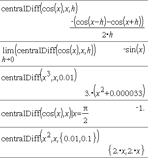
You are here: TI‑Nspire™ CX CAS Reference Guide > Alphabetical Listing > C

C

ceiling(Expr1) integer

Returns the nearest integer that is the argument.

The argument can be a real or a complex number.

Note: See also floor().

ceiling(List1) list
ceiling(Matrix1) matrix

Returns a list or matrix of the ceiling of each element.

centralDiff()

centralDiff(Expr1,Var [=Value][,Step]) expression

centralDiff(Expr1,Var [,Step])|Var=Value expression

centralDiff(Expr1,Var [=Value][,List]) list

centralDiff(List1,Var [=Value][,Step]) list

centralDiff(Matrix1,Var [=Value][,Step]) matrix

Returns the numerical derivative using the central difference quotient formula.

When Value is specified, it overrides any prior variable assignment or any current “|” substitution for the variable.

Step is the step value. If Step is omitted, it defaults to 0.001.

When using List1 or Matrix1, the operation gets mapped across the values in the list or across the matrix elements.

Note: See also avgRC() and d().

cFactor()

cFactor(Expr1[,Var]) expression
cFactor(List1[,Var]) list
cFactor(Matrix1[,Var]) matrix

cFactor(Expr1) returns Expr1 factored with respect to all of its variables over a common denominator.

Expr1 is factored as much as possible toward linear rational factors even if this introduces new non-real numbers. This alternative is appropriate if you want factorization with respect to more than one variable.

cFactor(Expr1,Var) returns Expr1 factored with respect to variable Var.

Expr1 is factored as much as possible toward factors that are linear in Var, with perhaps non-real constants, even if it introduces irrational constants or subexpressions that are irrational in other variables.

The factors and their terms are sorted with Var as the main variable. Similar powers of Var are collected in each factor. Include Var if factorization is needed with respect to only that variable and you are willing to accept irrational expressions in any other variables to increase factorization with respect to Var. There might be some incidental factoring with respect to other variables.

For the Auto setting of the Auto or Approximate mode, including Var also permits approximation with floating-point coefficients where irrational coefficients cannot be explicitly expressed concisely in terms of the built-in functions. Even when there is only one variable, including Var might yield more complete factorization.

Note: See also factor().

To see the entire result,
press 5 and then use 7 and 8 to move the cursor.

char()

char(Integer) character

Returns a character string containing the character numbered Integer from the handheld character set. The valid range for Integer is 0–65535.

charPoly()

charPoly(squareMatrix,Var) polynomial expression

charPoly(squareMatrix,Expr) polynomial expression

charPoly(squareMatrix1,Matrix2) polynomial expression

Returns the characteristic polynomial of squareMatrix. The characteristic polynomial of n×n matrix A, denoted by pA(λ), is the polynomial defined by

pA(λ) = det(λIA)

where I denotes the n×n identity matrix.

squareMatrix1 and squareMatrix2 must have the equal dimensions.

χ22way

χ22way obsMatrix

chi22way obsMatrix

Computes a χ2 test for association on the two-way table of counts in the observed matrix obsMatrix. A summary of results is stored in the stat.results variable. (here)

For information on the effect of empty elements in a matrix, see “Empty (Void) Elements,” here.


Output variable

Description

stat.χ2

Chi square stat: sum (observed - expected)2/expected

stat.PVal

Smallest level of significance at which the null hypothesis can be rejected

stat.df

Degrees of freedom for the chi square statistics

stat.ExpMat

Matrix of expected elemental count table, assuming null hypothesis

stat.CompMat

Matrix of elemental chi square statistic contributions

χ2Cdf()

χ2Cdf(lowBound,upBound,df) number if lowBound and upBound are numbers, list if lowBound and upBound are lists

chi2Cdf(lowBound,upBound,df) number if lowBound and upBound are numbers, list if lowBound and upBound are lists

Computes the χ2 distribution probability between lowBound and upBound for the specified degrees of freedom df.

For P(X upBound), set lowBound = 0.

For information on the effect of empty elements in a list, see “Empty (Void) Elements,” here.


χ2GOF

χ2GOF obsList,expList,df

chi2GOF obsList,expList,df

Performs a test to confirm that sample data is from a population that conforms to a specified distribution. obsList is a list of counts and must contain integers. A summary of results is stored in the stat.results variable. (See here.)

For information on the effect of empty elements in a list, see “Empty (Void) Elements,” here.


Output variable

Description

stat.χ2

Chi square stat: sum((observed - expected)2/expected

stat.PVal

Smallest level of significance at which the null hypothesis can be rejected

stat.df

Degrees of freedom for the chi square statistics

stat.CompList

Elemental chi square statistic contributions

χ2Pdf()

χ2Pdf(XVal,df) number if XVal is a number, list if XVal is a list

chi2Pdf(XVal,df) number if XVal is a number, list if XVal is a list

Computes the probability density function (pdf) for the χ2 distribution at a specified XVal value for the specified degrees of freedom df.

For information on the effect of empty elements in a list, see “Empty (Void) Elements,” here.


ClearAZ

ClearAZ

Clears all single-character variables in the current problem space.

If one or more of the variables are locked, this command displays an error message and deletes only the unlocked variables. See unLock, here.

ClrErr

ClrErr

Clears the error status and sets system variable errCode to zero.

The Else clause of the Try...Else...EndTry block should use ClrErr or PassErr. If the error is to be processed or ignored, use ClrErr. If what to do with the error is not known, use PassErr to send it to the next error handler. If there are no more pending Try...Else...EndTry error handlers, the error dialog box will be displayed as normal.

Note: See also PassErr, here, and Try, here.

Note for entering the example: For instructions on entering multi-line program and function definitions, refer to the Calculator section of your product guidebook.

For an example of ClrErr, See Example 2 under the Try command, here.


colAugment()

colAugment(Matrix1, Matrix2) matrix

Returns a new matrix that is Matrix2 appended to Matrix1. The matrices must have equal column dimensions, and Matrix2 is appended to Matrix1 as new rows. Does not alter Matrix1 or Matrix2.

colDim()

colDim(Matrix) expression

Returns the number of columns contained in Matrix.

Note: See also rowDim().

colNorm()

colNorm(Matrix) expression

Returns the maximum of the sums of the absolute values of the elements in the columns in Matrix.

Note: Undefined matrix elements are not allowed. See also rowNorm().

comDenom()

comDenom(Expr1[,Var]) expression
comDenom(List1[,Var]) list
comDenom(Matrix1[,Var]) matrix

comDenom(Expr1) returns a reduced ratio of a fully expanded numerator over a fully expanded denominator.

comDenom(Expr1,Var) returns a reduced ratio of numerator and denominator expanded with respect to Var. The terms and their factors are sorted with Var as the main variable. Similar powers of Var are collected. There might be some incidental factoring of the collected coefficients. Compared to omitting Var, this often saves time, memory, and screen space, while making the expression more comprehensible. It also makes subsequent operations on the result faster and less likely to exhaust memory.

If Var does not occur in Expr1, comDenom(Expr1,Var) returns a reduced ratio of an unexpanded numerator over an unexpanded denominator. Such results usually save even more time, memory, and screen space. Such partially factored results also make subsequent operations on the result much faster and much less likely to exhaust memory.

Even when there is no denominator, the comden function is often a fast way to achieve partial factorization if factor() is too slow or if it exhausts memory.

Hint: Enter this comden() function definition and routinely try it as an alternative to comDenom() and factor().


completeSquare ()

completeSquare(ExprOrEqn, Var) expression or equation

completeSquare(ExprOrEqn, Var^Power) expression or equation

completeSquare(ExprOrEqn, Var1, Var2 [,...]) expression or equation

completeSquare(ExprOrEqn, {Var1, Var2 [,...]}) expression or equation

Converts a quadratic polynomial expression of the form ax2+bx+c into the form a(x-h)2+k

- or -

Converts a quadratic equation of the form ax2+bx+c=d into the form a(x-h)2=k

The first argument must be a quadratic expression or equation in standard form with respect to the second argument.

The Second argument must be a single univariate term or a single univariate term raised to a rational power, for example x, y2, or z(1/3).

The third and fourth syntax attempt to complete the square with respect to variables Var1, Var2 [,… ]).

conj()

conj(Expr1) expression

conj(List1) list

conj(Matrix1) matrix

Returns the complex conjugate of the argument.

Note: All undefined variables are treated as real variables.

constructMat()

constructMat(Expr,Var1,Var2,numRows,numCols) matrix

Returns a matrix based on the arguments.

Expr is an expression in variables Var1 and Var2. Elements in the resulting matrix are formed by evaluating Expr for each incremented value of Var1 and Var2.

Var1 is automatically incremented from 1 through numRows. Within each row, Var2 is incremented from 1 through numCols.

CopyVar

CopyVar Var1, Var2

CopyVar Var1., Var2.

CopyVar Var1, Var2 copies the value of variable Var1 to variable Var2, creating Var2 if necessary. Variable Var1 must have a value.

If Var1 is the name of an existing user-defined function, copies the definition of that function to function Var2. Function Var1 must be defined.

Var1 must meet the variable-naming requirements or must be an indirection expression that simplifies to a variable name meeting the requirements.

CopyVar Var1., Var2. copies all members of the Var1. variable group to the Var2. group, creating Var2. if necessary.

Var1. must be the name of an existing variable group, such as the statistics stat.nn results, or variables created using the LibShortcut() function. If Var2. already exists, this command replaces all members that are common to both groups and adds the members that do not already exist. If one or more members of Var2. are locked, all members of Var2. are left unchanged.

corrMat()

corrMat(List1,List2[,…[,List20]])

Computes the correlation matrix for the augmented matrix [List1, List2, ..., List20].


cos

Expr cos

Note: You can insert this operator from the computer keyboard by typing @>cos.

Represents Expr in terms of cosine. This is a display conversion operator. It can be used only at the end of the entry line.

cos reduces all powers of
    sin(...) modulo 1cos(...)^2
so that any remaining powers of cos(...) have exponents in the range (0, 2). Thus, the result will be free of sin(...) if and only if sin(...) occurs in the given expression only to even powers.

Note: This conversion operator is not supported in Degree or Gradian Angle modes. Before using it, make sure that the Angle mode is set to Radians and that Expr does not contain explicit references to degree or gradian angles.


cos()

cos(Expr1) expression

cos(List1) list

cos(Expr1) returns the cosine of the argument as an expression.

cos(List1) returns a list of the cosines of all elements in List1.

Note: The argument is interpreted as a degree, gradian or radian angle, according to the current angle mode setting. You can use °G, or r to override the angle mode temporarily.

In Degree angle mode:

In Gradian angle mode:


In Radian angle mode:

cos(squareMatrix1) squareMatrix

Returns the matrix cosine of squareMatrix1. This is not the same as calculating the cosine of each element.

When a scalar function f(A) operates on squareMatrix1 (A), the result is calculated by the algorithm:

Compute the eigenvalues (λi) and eigenvectors (Vi) of A.

squareMatrix1 must be diagonalizable. Also, it cannot have symbolic variables that have not been assigned a value.

Form the matrices:

Then A = X B X¹ and f(A) = X f(B) X¹. For example, cos(A) = X cos(B) X¹ where:

cos(B) =


All computations are performed using floating-point arithmetic.

In Radian angle mode:

cos¹()

cos¹(Expr1) expression

cos¹(List1) list

cos¹(Expr1) returns the angle whose cosine is Expr1 as an expression.

cos¹(List1) returns a list of the inverse cosines of each element of List1.

Note: The result is returned as a degree, gradian or radian angle, according to the current angle mode setting.

Note: You can insert this function from the keyboard by typing arccos(...).

In Degree angle mode:


In Gradian angle mode:


In Radian angle mode:

cos¹(squareMatrix1) squareMatrix

Returns the matrix inverse cosine of squareMatrix1. This is not the same as calculating the inverse cosine of each element. For information about the calculation method, refer to cos().

squareMatrix1 must be diagonalizable. The result always contains floating-point numbers.

In Radian angle mode and Rectangular Complex Format:

To see the entire result,
press 5 and then use 7 and 8 to move the cursor.

cosh()

cosh(Expr1) expression

cosh(List1) list

cosh(Expr1) returns the hyperbolic cosine of the argument as an expression.

cosh(List1) returns a list of the hyperbolic cosines of each element of List1.

In Degree angle mode:

cosh(squareMatrix1) squareMatrix

Returns the matrix hyperbolic cosine of squareMatrix1. This is not the same as calculating the hyperbolic cosine of each element. For information about the calculation method, refer to cos().

squareMatrix1 must be diagonalizable. The result always contains floating-point numbers.

In Radian angle mode:

cosh¹()

cosh¹(Expr1) expression

cosh¹(List1) list

cosh¹(Expr1) returns the inverse hyperbolic cosine of the argument as an expression.

cosh¹(List1) returns a list of the inverse hyperbolic cosines of each element of List1.

Note: You can insert this function from the keyboard by typing arccosh(...).

cosh¹(squareMatrix1) squareMatrix

Returns the matrix inverse hyperbolic cosine of squareMatrix1. This is not the same as calculating the inverse hyperbolic cosine of each element. For information about the calculation method, refer to cos().

squareMatrix1 must be diagonalizable. The result always contains floating-point numbers.

In Radian angle mode and In Rectangular Complex Format:

To see the entire result,
press 5 and then use 7 and 8 to move the cursor.

cot()

cot(Expr1) expression

cot(List1) list

Returns the cotangent of Expr1 or returns a list of the cotangents of all elements in List1.

Note: The argument is interpreted as a degree, gradian or radian angle, according to the current angle mode setting. You can use °G, or r to override the angle mode temporarily.

In Degree angle mode:


In Gradian angle mode:


In Radian angle mode:

cot⁻¹()

cot⁻¹(Expr1) expression

cot¹(List1) list

Returns the angle whose cotangent is Expr1 or returns a list containing the inverse cotangents of each element of List1.

Note: The result is returned as a degree, gradian or radian angle, according to the current angle mode setting.

Note: You can insert this function from the keyboard by typing arccot(...).

In Degree angle mode:


In Gradian angle mode:


In Radian angle mode:

coth()

coth(Expr1) expression

coth(List1) list

Returns the hyperbolic cotangent of Expr1 or returns a list of the hyperbolic cotangents of all elements of List1.

coth¹()

coth¹(Expr1) expression

coth¹(List1) list

Returns the inverse hyperbolic cotangent of Expr1 or returns a list containing the inverse hyperbolic cotangents of each element of List1.

Note: You can insert this function from the keyboard by typing arccoth(...).

count()

count(Value1orList1 [,Value2orList2 [,...]]) value

Returns the accumulated count of all elements in the arguments that evaluate to numeric values.

Each argument can be an expression, value, list, or matrix. You can mix data types and use arguments of various dimensions.

For a list, matrix, or range of cells, each element is evaluated to determine if it should be included in the count.

Within the Lists & Spreadsheet application, you can use a range of cells in place of any argument.

Empty (void) elements are ignored. For more information on empty elements, see here.


In the last example, only 1/2 and 3+4*i are counted. The remaining arguments, assuming x is undefined, do not evaluate to numeric values.

countif()

countif(List,Criteria) value

Returns the accumulated count of all elements in List that meet the specified Criteria.

Criteria can be:

A value, expression, or string. For example, 3 counts only those elements in List that simplify to the value 3.
A Boolean expression containing the symbol ? as a placeholder for each element. For example, ?<5 counts only those elements in List that are less than 5.

Within the Lists & Spreadsheet application, you can use a range of cells in place of List.

Empty (void) elements in the list are ignored. For more information on empty elements, see here.

Note: See also sumIf(), here, and frequency(), here.

Counts the number of elements equal to 3.


Counts the number of elements equal to “def.”


Counts the number of elements equal to x; this example assumes the variable x is undefined.

Counts 1 and 3.


Counts 3, 5, and 7.


Counts 1, 3, 7, and 9.

cPolyRoots()

cPolyRoots(Poly,Var) list

cPolyRoots(ListOfCoeffs) list

The first syntax, cPolyRoots(Poly,Var), returns a list of complex roots of polynomial Poly with respect to variable Var.

Poly must be a polynomial in one variable.

The second syntax, cPolyRoots(ListOfCoeffs), returns a list of complex roots for the coefficients in ListOfCoeffs.

Note: See also polyRoots(), here.


crossP()

crossP(List1, List2) list

Returns the cross product of List1 and List2 as a list.

List1 and List2 must have equal dimension, and the dimension must be either 2 or 3.

crossP(Vector1, Vector2) vector

Returns a row or column vector (depending on the arguments) that is the cross product of Vector1 and Vector2.

Both Vector1 and Vector2 must be row vectors, or both must be column vectors. Both vectors must have equal dimension, and the dimension must be either 2 or 3.

csc()

csc(Expr1) expression

csc(List1) list

Returns the cosecant of Expr1 or returns a list containing the cosecants of all elements in List1.

In Degree angle mode:


In Gradian angle mode:


In Radian angle mode:

csc¹()

csc¹(Expr1) expression

csc¹(List1) list

Returns the angle whose cosecant is Expr1 or returns a list containing the inverse cosecants of each element of List1.

Note: The result is returned as a degree, gradian or radian angle, according to the current angle mode setting.

Note: You can insert this function from the keyboard by typing arccsc(...).

In Degree angle mode:


In Gradian angle mode:


In Radian angle mode:

csch()

csch(Expr1) expression

csch(List1) list

Returns the hyperbolic cosecant of Expr1 or returns a list of the hyperbolic cosecants of all elements of List1.

csch¹()

csch¹(Expr1) expression

csch¹(List1) list

Returns the inverse hyperbolic cosecant of Expr1 or returns a list containing the inverse hyperbolic cosecants of each element of List1.

Note: You can insert this function from the keyboard by typing arccsch(...).

cSolve()

cSolve(Equation, Var) Boolean expression

cSolve(Equation, Var=Guess) Boolean expression

cSolve(Inequality, Var) Boolean expression


Returns candidate complex solutions of an equation or inequality for Var. The goal is to produce candidates for all real and non-real solutions. Even if Equation is real, cSolve() allows non-real results in Real result Complex Format.

Although all undefined variables that do not end with an underscore (_) are processed as if they were real, cSolve() can solve polynomial equations for complex solutions.

cSolve() temporarily sets the domain to complex during the solution even if the current domain is real. In the complex domain, fractional powers having odd denominators use the principal rather than the real branch. Consequently, solutions from solve() to equations involving such fractional powers are not necessarily a subset of those from cSolve().

cSolve() starts with exact symbolic methods. cSolve() also uses iterative approximate complex polynomial factoring, if necessary.

Note: See also cZeros(), solve(), and zeros().

In Display Digits mode of Fix 2:

To see the entire result,
press 5 and then use 7 and 8 to move the cursor.

cSolve(Eqn1andEqn2 [and],
VarOrGuess1, VarOrGuess2 [, … ]) Boolean expression

cSolve(SystemOfEqns, VarOrGuess1,
VarOrGuess2 [, …]) Boolean expression

Returns candidate complex solutions to the simultaneous algebraic equations, where each varOrGuess specifies a variable that you want to solve for.

Optionally, you can specify an initial guess for a variable. Each varOrGuess must have the form:

variable
– or –
variable = real or non-real number

For example, x is valid and so is x=3+i.


If all of the equations are polynomials and if you do NOT specify any initial guesses, cSolve() uses the lexical Gröbner/Buchberger elimination method to attempt to determine all complex solutions.

Complex solutions can include both real and non-real solutions, as in the example to the right.

To see the entire result,
press 5 and then use 7 and 8 to move the cursor.

Simultaneous polynomial equations can have extra variables that have no values, but represent given numeric values that could be substituted later.

To see the entire result,
press 5 and then use 7 and 8 to move the cursor.

You can also include solution variables that do not appear in the equations. These solutions show how families of solutions might contain arbitrary constants of the form ck, where k is an integer suffix from 1 through 255.

For polynomial systems, computation time or memory exhaustion may depend strongly on the order in which you list solution variables. If your initial choice exhausts memory or your patience, try rearranging the variables in the equations and/or varOrGuess list.

To see the entire result,
press 5 and then use 7 and 8 to move the cursor.

If you do not include any guesses and if any equation is non-polynomial in any variable but all equations are linear in all solution variables, cSolve() uses Gaussian elimination to attempt to determine all solutions.

If a system is neither polynomial in all of its variables nor linear in its solution variables, cSolve() determines at most one solution using an approximate iterative method. To do so, the number of solution variables must equal the number of equations, and all other variables in the equations must simplify to numbers.

A non-real guess is often necessary to determine a non-real solution. For convergence, a guess might have to be rather close to a solution.

To see the entire result,
press 5 and then use 7 and 8 to move the cursor.

CubicReg

CubicReg X, Y[, [Freq] [, Category, Include]]

Computes the cubic polynomial regression y=ax3+bx2+cx+d on lists X and Y with frequency Freq. A summary of results is stored in the stat.results variable. (See here.)

All the lists must have equal dimension except for Include.

X and Y are lists of independent and dependent variables.

Freq is an optional list of frequency values. Each element in Freq specifies the frequency of occurrence for each corresponding X and Y data point. The default value is 1. All elements must be integers 0.

Category is a list of category codes for the corresponding X and Y data.

Include is a list of one or more of the category codes. Only those data items whose category code is included in this list are included in the calculation.

For information on the effect of empty elements in a list, see “Empty (Void) Elements,” here.


Output variable

Description

stat.RegEqn

Regression equation: ax3+bx2+cx+d

stat.a, stat.b, stat.c, stat.d

Regression coefficients

stat.R2

Coefficient of determination

stat.Resid

Residuals from the regression

stat.XReg

List of data points in the modified X List actually used in the regression based on restrictions of Freq, Category List, and Include Categories

stat.YReg

List of data points in the modified Y List actually used in the regression based on restrictions of Freq, Category List, and Include Categories

stat.FreqReg

List of frequencies corresponding to stat.XReg and stat.YReg

cumulativeSum()

cumulativeSum(List1) list

Returns a list of the cumulative sums of the elements in List1, starting at element 1.

cumulativeSum(Matrix1) matrix

Returns a matrix of the cumulative sums of the elements in Matrix1. Each element is the cumulative sum of the column from top to bottom.

An empty (void) element in List1 or Matrix1 produces a void element in the resulting list or matrix. For more information on empty elements, see here.

Cycle

Cycle

Transfers control immediately to the next iteration of the current loop (For, While, or Loop).

Cycle is not allowed outside the three looping structures (For, While, or Loop).

Note for entering the example: For instructions on entering multi-line program and function definitions, refer to the Calculator section of your product guidebook.

Function listing that sums the integers from 1 to 100 skipping 50.

Cylind

Vector Cylind

Note: You can insert this operator from the computer keyboard by typing @>Cylind.

Displays the row or column vector in cylindrical form [r,θ, z].

Vector must have exactly three elements. It can be either a row or a column.


cZeros()

cZeros(Expr, Var) list

Returns a list of candidate real and non-real values of Var that make Expr=0. cZeros() does this by computing
explist(cSolve(Expr=0,Var),Var). Otherwise, cZeros() is similar to zeros().

Note: See also cSolve(), solve(), and zeros().

In Display Digits mode of Fix 3:

To see the entire result,
press 5 and then use 7 and 8 to move the cursor.

cZeros({Expr1, Expr2[, … ] },
  {VarOrGuess1,VarOrGuess2[, … ] }) matrix

Returns candidate positions where the expressions are zero simultaneously. Each VarOrGuess specifies an unknown whose value you seek.


Optionally, you can specify an initial guess for a variable. Each VarOrGuess must have the form:

variable
– or –
variable = real or non-real number

For example, x is valid and so is x=3+i.


If all of the expressions are polynomials and you do NOT specify any initial guesses, cZeros() uses the lexical Gröbner/Buchberger elimination method to attempt to determine all complex zeros.

Complex zeros can include both real and non-real zeros, as in the example to the right.

Each row of the resulting matrix represents an alternate zero, with the components ordered the same as the VarOrGuess list. To extract a row, index the matrix by [row].

Extract row 2:

Simultaneous polynomials can have extra variables that have no values, but represent given numeric values that could be substituted later.

You can also include unknown variables that do not appear in the expressions. These zeros show how families of zeros might contain arbitrary constants of the form ck, where k is an integer suffix from 1 through 255.

For polynomial systems, computation time or memory exhaustion may depend strongly on the order in which you list unknowns. If your initial choice exhausts memory or your patience, try rearranging the variables in the expressions and/or VarOrGuess list.

If you do not include any guesses and if any expression is non-polynomial in any variable but all expressions are linear in all unknowns, cZeros() uses Gaussian elimination to attempt to determine all zeros.

If a system is neither polynomial in all of its variables nor linear in its unknowns, cZeros() determines at most one zero using an approximate iterative method. To do so, the number of unknowns must equal the number of expressions, and all other variables in the expressions must simplify to numbers.

A non-real guess is often necessary to determine a non-real zero. For convergence, a guess might have to be rather close to a zero.