In this lesson you will explore finding absolute and local extreme values of a function using the TI-89. The standard first and second derivative tests will be used to find and identify local extreme values of a function.

• Before beginning this lesson execute the NewProb command from the F6:Clean Up Menu

Absolute Extreme Values of a Function

Let f be a function with domain D. Then f(c) is the

(a) absolute maximum value of f on D if and only if f(x) f(c) for all x in D.

(b) absolute minimum value of f on D if and only if f(x) f(c) for all x in D.

Finding the Absolute Extreme Values of f(x) = x²

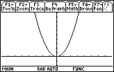
The graph of f in the figure below suggests that f has no absolute maximum value and has an absolute minimum of 0 at x = 0.

Finding the Absolute Extreme Values of f(x) = x² on [-2, 3]

The graph of f in the window [-2, 3] suggests that f has an absolute maximum of 9 at x = 3 and an absolute minimum of 0 at x = 0.

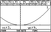
This example suggests that existence of absolute extrema depends on the domain of the function.

Extreme Value Theorem

This important theorem can guide our investigations when we search for absolute extreme values of a function.

Theorem 1 If f is continuous on a closed interval [a, b], then f has both an absolute maximum value and an absolute minimum value on the interval.

Local Extreme Values of a Function

Let c be an interior point of the domain of the function f. Then f has a

(a) local maximum at c if and only if f(x) f(c) for all x in some open interval containing c.

(b) local minimum at c if and only if f(x) f(c) for all x in some open interval containing c.

We can extend the definition of local extrema to endpoints of intervals. A function f has a local maximum or local minimum at an endpoint c if the appropriate inequality holds for all x in some half-open domain interval containing c.

The following theorem helps us find candidates for local extreme values of a function.

Theorem 2 If a function has a local maximum value or a local minimum value at an interior point c of its domain and if f ' exists at c, then f ' (c) = 0.

We can see from the graph of f(x) = x² above that f has a local minimum of 0 at x = 0. We observed that f has no absolute maximum value but we can also see that f has no local maximum value either.

Finding Extreme Values of a Function

Because of Theorem 2, we usually need to look at only a few points to find a function's extreme values. Those points consist of interior domain points where f ' = 0 or where f ' does not exist and the domain endpoints which are not covered by the theorem.

Critical Points

A critical point is an interior point in the domain of a function at which f ' (x) = 0 or f ' (x) does not exist.

Find the Extreme Values of f(x) = x² on [-2, 3]

Refer to the graph of f above.

• Because f ' exists at all values of f in [-2, 3] and f '(x) = 2x is zero only at x = 0, 0 is the only critical point of f.
• The values of f at the endpoints are f(-2) = 4 and f(3) = 9.
• f has a local minimum of 0 at x = 0 which is also an absolute minimum.
• f has a local maximum of 4 at x = -2 and a local maximum of 9 at x = 3. The absolute maximum of f is 9.

11.1.1 Draw the graph and find the extreme values of f(x) = x² on [-4, 2].
Click here for the answer.

Find the Extreme Values of f(x) = x^2/3 on [-2, 4]

• Draw the graph of f in [-2, 4] x [-1, 3]. Enter x^2/3 in y1(x).

• Use the home screen derivative command to find f '.

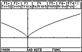
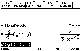
We can see that f ' does not exist at x = 0 and is not equal to 0 anywhere on [-2, 4]. The only critical point of f is at x = 0.

Find the value of f at the endpoints.
From the graph of f press and select 1:Value to evaluate f at x = -2 and x = 4, as shown in the screens below.

 

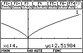
f has a local and absolute minimum of 0 at 0. The value of f at x = -2 is approximately 1.587 and the value at x = 4 is appoximately 2.520. The absolute maximum value of f is approximately 2.520 at x = 4.

Find the Extreme Values of f(x) = x³ – 2x – 2 cosx

• Define f(x) = x³ – 2x – 2 cos x.
  The domains of f and f ' are both the set of all real numbers, so there are no values at which f ' doesn't exist and there are no endpoints to consider.
  Enter f(x) into y1 and f '(x) into y2.
  Set the graphing style of y1 to thick and graph the two functions in [-5, 5] x [-5, 5]
 

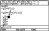
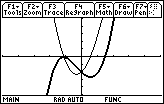
We can see from the graph that f '(x) has a negative zero and a positive zero. Because the sign of f'(x) goes from positive to negative at the negative zero of f '(x), the first derivative test for extreme values tell us that the function f has a local maximum value at this value of x. Similarly, the sign of f '(x) goes from negative to positive at the positive zero of f '(x), so the first derivative test tells us that the function f has a local minimum value at this value of x.

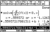
We next approximate the zeros of f ' on the home screen as shown in the screen below.

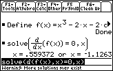
The positive zero is approximately 0.559 and the negative zero is approximately -1.263.

• Store the negative zero of f ' in a and the positive value in b.
• Begin by pasting the two zeros found above to the Edit Line.
• Delete the two "x=" and the word "or" by using the backspace key .
• Place the cursor at the end of the negative number and press [A].
• Place the cursor at the end of the positive number and press [B].
• Insert the colon key (the alpha feature above ) immediately to the left of the negative number.
• Finally, delete any blank spaces.
• The Edit Line should look like the following:
  
  
• Press

According to the second derivative test for extreme values, the value of f at a zero of f ' is

• (a) a local maximum if f " < 0 at that value of x, and
• (b) a local minimum if f " > 0 at that value of x.

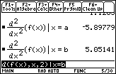
The figure below calculates the value of f " at x = a and x = b, and supports our earlier observations.

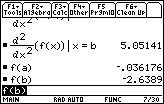
• We know that and , so f has neither an absolute maximum or absolute minimum. However, f has a local maximum value of approximately -0.036 at x -1.263 and a local minimum value of approximately -2.639 at x 0.559. See the figure below.

You can use these techniques in Lessons 11.2-11.4.