In Lesson 7.1 you found average velocities over different time intervals. In this lesson you will find the instantaneous velocity of the falling object at t = 0.16. Each of the average velocities found in Lesson 7.1 could be considered an approximation of the instantaneous velocity at t = 0.16, but none was exact.

Getting Better Approximations

You can use the average velocity function you defined in Lesson 7.1 to find a series of approximations that will lead to the instantaneous velocity of an object at a given instant.

7.2.1 Use the function avel you defined in Lesson 7.1 to enter the average velocities over the intervals near t = 0.16 indicated by the following data points, and use DrawSlp to draw the corresponding lines on the scatter plot. Click here for the answer.

Data Points	Average Velocity
(0.16, 0.716) to (0.26, 0.506)
(0.16, 0.716) to (0.22, 0.600)
(0.16, 0.716) to (0.18, 0.681)

7.2.2 Which of the three average velocities is the best approximation to the instantaneous velocity? Why? Click here for the answer.

• Clear the average velocity lines from the scatter plot by pressing

Fitting a Curve to the Data

The smaller the elapsed time interval, the better the average velocity approximates the instantaneous velocity. The smallest interval near t = 0.16 provided by the data is 0.02. However, if you could find a continuous curve through the scatter plot, you could find points on the curve even closer to (0.16, 0.716) that could be used to find even better approximations of the instantaneous velocity there. A regression curve for the data can provide such approximate data points.

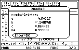
• Use QuadReg in the F4:Calc Regression menu of the Statistics/List Editor to find a second degree polynomial that fits the scatter plot and store it in y1 in the Y= Editor Click here to review Keystrokes to create a regression equation.

Set up Screen for Quadratic Regression	The regression equation is y –4.503x2 –.209x + .864

• Display the regression equation with the scatter plot by pressing

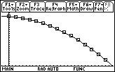
Using the Regression Equation

The height of the book at t = 0.16 and t = 0.18 can now be approximated by finding y1(0.18) and y1(0.16). These values may be used to approximate the average velocity by computing

• Find the approximate average velocity over the interval t = 0.16 and t = 0.18 by entering the command (y1(0.18)–y1(0.16))/(0.18–0.16)

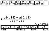
This result is a good approximation of the average velocity of -1.75 you found in Question 7.2.2 using the table data values over the same interval.

Finding Even Better Approximations

Points even closer to (0.16, 0.716) may be found by using the quadratic function stored in y1.

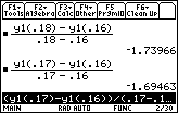
Find the average velocity for the interval from t = 0.16 and t = 0.17.

• Evaluate (y1(0.17)–y1(0.16))/(0.17–0.16) by editing the command in the Edit Line

7.2.3 Using the regression equation in y1, find the average velocities for the following smaller and smaller time intervals.

t = 0.16 to t = 0.161 (elapsed time = 0.001 seconds)

t = 0.16 to t = 0.1601 (elapsed time = 0.0001 seconds)

t = 0.16 to t = 0.16001 (elapsed time =0 .00001 seconds)

Click here for the answer.

Finding Instantaneous Velocity

As the elapsed time approaches zero, the average velocities approach a limiting value. This limit is the instantaneous velocity, which can be found by letting h represent the elapsed time and evaluating

• Evaluate limit((y1(0.16+h)–y1(0.16)) / h, h, 0)

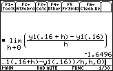
The instantaneous velocity at t = 0.16 is –1.6496 m/s.

Calculating the limit of the difference quotient To find the instantaneous velocity above we calculated the limit of the following difference quotient Because the quadratic function y had non-integer, decimal coefficients this TI-89 procedure can fail to find a limit even when a limit exists if the TI-89 is set in AUTO mode. It, of course, did not fail above. To resolve this difficulty put the TI-89 in EXACT mode to calculate the limit. If the limit exists it generally is a complicated rational number. Use the approx( command from the catalog to approximate the exact value found. Note that pressing in AUTO mode will also fail. This is what will happen in Question 6 of the Self Test if you use this procedure.

Visualizing Instantaneous Velocity

A special line is associated with the instantaneous velocity.

• Draw the line associated with instantaneous velocity by entering the command DrawSlp 0.16, 0.716, –1.6496

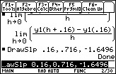
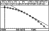
	Visualizing the instantaneous velocity

The line is

A tangent line to the graph of f at the point (a, f(a)) is the line through (a, f(a)) with slope , provided that the limit exists.

tangent to the curve at (0.16, 0.716), and the slope of the tangent line to the curve at the point where x = 0.16 is the instantaneous velocity.