In this lesson you will use the TI-89 to find an equation that fits the logistic scatter plot created in Lesson 3.1.

Open the Stats/List Editor

• Display the Flash Applications menu by pressing
• Highlight "Stats/List Editor" using the cursor movement keys
• Open the Stats/List Editor by pressing

The data from Lesson 3.1 should still be in list1 and list2.

Calculate the Logistic Regression Equation

• Display the "Calc" menu by pressing

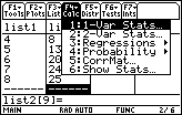
The third option in this menu is "Regressions".

• Display the regression submenu by using the cursor movement keys

There are many types of functions in this submenu.

• Scroll down with the cursor movement keys and highlight "B:Logistic"

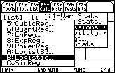
• Open the Logistic Regression dialog box by pressing

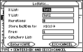
In this dialog box you will specify the x and y values and designate where the logistic regression equation will be stored.

The entry in the "X List" box should be "list1." If it is not, click here to see keystroke instructions to enter list1.

The entry in the "Y List" box should be list2. If you would like to see keystroke instructions to enter list2 in this box click here.
Leave "iterations" set at 8.

Finding Stored Variables If you have many variables stored on your calculator making it hard to scroll to a certain variable like "list1", there are two other options available. You can simply type the name of the variable where you need it, or After pressing [VAR-LINK] press to go to the VAR-LINK VIEW. Then choose [3:List] as the Var Type and press . Now choose the list desired. This feature sorts the variables into types.

Store the Regression Equation into the Y= Editor

The entry beside "Store RegEqn to:" should be y1(x). This will store the regression equation in y1 in the Y= Editor. If the entry shown in the logistic dialog box is not y1, you should change the selection. Note that if your calculator has a function stored in y1, it will be overwritten and lost. Click here to see keystroke instructions to store the regression equation in y1.

When the values for the Logistic dialog box have been properly selected

• Compute the regression equation by pressing

This may take several minutes. You should see a busy indicator in the lower right corner of the screen while the regression coefficients are being calculated. When the calculations are finished, the coefficients will be displayed.

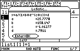
The form of the logistic regression equation chosen is , as shown at the top of the screen, and the values for the coefficients a, b, c, and d are shown below the equation.

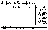
Residuals

• Close the coefficient box and return to the Stats/List Editor by pressing

Notice that a new column containing the

A residual is a measure of the error between an actual data value and the corresponding value given by an equation. That is, the residual is d – y where (x, d) is the data point and (x, y) is the point determined by the equation.

residuals has been inserted in the Stats/List Editor. We will not do anything with the residuals at this time.

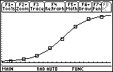
Graph the Regression Equation

The logistic regression equation is stored in y1. To see how well the graph of the equation fits the scatter plot,

• Display the graph screen by pressing [GRAPH]

3.2.1 Write the equation that is shown by y1 in the Y= editor. Click here for the answer.