Solutions to differential equations are found graphically and numerically in this lesson. Slope fields and particular solutions are also discussed.

The TI-89 has a graphing mode that allows you to find graphical and numerical solutions to differential equations. This mode is called the Differential Equation graphing mode.

Solve y' = 2x graphically.

• Open the Mode dialog box by pressing
• Open the Graph submenu by pressing
• Highlight "6:DIFF EQUATIONS"

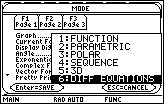
• Select and save this mode setting by pressing twice

The Differential Equation Mode Variable The independent variable used in Differential Equation graphing mode is t. In order to enter the differential equation y' = 2x you must enter 2t instead of 2x.

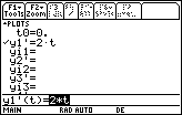
• Enter the equation y1' = 2·t into the Y= Editor

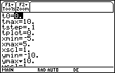
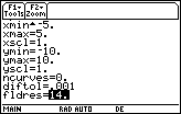
• Select the window values shown below

 

Window Parameters The new relevant parameters shown in the Window Editor are listed below. t0 indicates the initial condition x-value entered in the Y= Editor. This will be discussed later in this lesson. tstep is used to determine the t values between tplot and tmax where points are plotted to graph solutions. tplot indicates the first t value plotted. fldres determines the number of columns used to draw a slope field across the full width of the screen.

• The graph that results from pressing is called a slope-field.

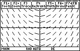
Slope Fields

The slope field contains short line segments with slope 2x at selected points in the window. This particular window uses 98 points arranged in 7 rows and 14 columns. The line segments could be thought of as linear approximations, or tangent lines, of particular solutions through the points.

Notice that all the line segments in a given column are parallel because they all have the same x-coordinate and therefore the same slope, 2x.

Finding a Particular Solution

Find the particular solution to the differential equation y' = 2x that satisfies the initial condition y(2) = 1.

• Display the Y= Editor
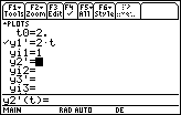
• y1' should be 2·t
• Move the cursor to "t0=" and enter 2
  This is the initial value of t, i.e., x.
• Move the cursor to "yi1="
  This is the value of y1 for the initial value t0: y1(t0) = yi1.
• Enter 1

• Press and set Fields to SLPFLD.
• Display the graph of the particular solution by pressing

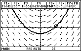
The slope field is shown and the particular solution when y(2) = 1 is indicated by the darker connected curve.

• Trace along the particular solution by pressing

The coordinates of t, x, and y will be displayed at the bottom of the screen.

18.4.1 Use the Trace feature to find y(3) for this particular solution.
Click here for the answer.

Creating a Table of Values

You can use the TI-89 Table feature to create a table of values for the particular solution to y' = 2x and y(2) = 1. The table will display a numerical representation of the solution to the initial-value problem.

• Open the Table Setup dialog box by pressing [TblSet]
• Set the values in dialog box so that tblStart = 0 and tbl = 1

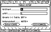
• Save these values by pressing
• Display the table by pressing [TABLE]

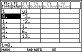
Each pair of values t and y1 represents a point (x, y) of the particular solution. Notice that the initial condition y(2) = 1 is shown and that y(3) = 6 is also there. You can display points on smaller intervals by adjusting tbl in the TblSet dialog box.

18.4.2 Graph the slope field and the solution for the initial-value problem y' = e^–x2 and y(-3) = 0.01. Use a [-3, 3] x [-0.5, 2] window. Remember to use t in place of x in the Y = Editor.
Click here for the answer.

The Slope Field of y' = y

The slope field for the differential equation y' = y is significantly different from those previously shown. The solution of y' = y represents a function where the slope of the tangent at each point (x, y) is the y-coordinate of that point. The slope of solutions to y' = y is a function of y rather than x. How do you think this will affect the slope field?

18.4.3 Sketch a rough approximation of the slope field for y' = y. Compare your slope field with the slope field given by your TI-89. What is the major difference between the slope field for this problem and the previously illustrated slope fields?
Click here for the answer.