Module 4 - Limit as x Approaches a

Module 4 - Limit as x Approaches a

Introduction | Lesson 1 | Lesson 2 | Lesson 3 | Self-Test

Lesson 4.1: Tolerances

A function can be described as a black box with an input and a corresponding output. Each input value x enters the box and then undergoes a transformation that produces a corresponding output value y. For continuous functions you can ensure that the output values will be close to a particular value of y if the input values are close enough to the corresponding value of x. In this lesson you will quantify the concept of closeness for a specific function.

Before you begin this lesson, perform the "New Problem" command and clear all graphs and plots in the Y= Editor.

Investigating Tolerances of y =

For y = , y is close to 2 when x is close to 3.

The key question is

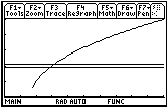
Begin the investigation by graphing the function and the two horizontal lines that represent the y-tolerances: one line that is 0.1 below y = 2 and the other line that is 0.1 above y = 2.

Graphing the Function and Output Bounds

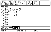
In the Y= Editor enter

The function: y1 =
The horizontal line 0.1 below 2: y2 = 2 – 0.1 = 1.9
The horizontal line 0.1 above 2: y3 = 2 + 0.1 = 2.1

Display the graph of the function to see its basic shape and the graphs of the two horizontal lines that represent the output tolerance. Display the window with xmin = 0, xmax = 10, xscl = 1, ymin = 0, ymax = 5, and yscl = 1.

A Better View

To better see the region of the graph where y is 0.1 unit away from 2, use viewing window values close to x = 3 and y = 2.

Define the window values by entering the values shown below

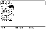
An abbreviation for this window is [2.8, 3.2] x [1.8, 2.2].

Display the graph by pressing [GRAPH]

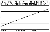
The graph of y = appears to be a diagonal line rather than a curve because a small portion of the graph has been magnified to fill this window. The points of intersection of the function and the lines have y-values that are 0.1 unit away from 2, and all points on the function between the two lines have y-values that are within 0.1 of 2.

Finding the x Tolerances Using the Intersection Feature

The x-coordinates of the points where the graph of the function intersects the horizontal lines determine how close x needs to be to 3 so that y is within 0.1 of 2. The "Intersection" feature in the Math menu of the Graph screen can be used to find the intersection points.

Display the Math menu by pressing

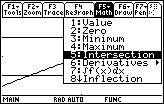
Select 5:Intersection

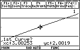
To find the x-value of the point of intersection of y2 = 1.9 (the lower bound of the y-tolerance) and
y1= (the graph of the function), you need to specify the two curves.

Selecting the Two Intersecting Curves

To find a point of intersection of two curves, the curves must be selected. The cursor is already on the function y1, as indicated by the small "1" in the upper right portion of the screen.

Select the function as one of the curves by pressing

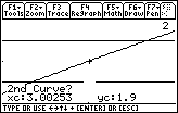
The small + shown on the graph of the function indicates that it is the first curve selected. The cursor is on the lower horizontal line to indicate that that line is currently chosen and it is blinking to indicate that it has not been selected. Note that "2" is shown in the upper right portion of the screen to indicate that the current position of the cursor is on the graph of y2.

Designate the lower line (y2) as the second curve by pressing

Specifying a Lower Bound

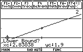
The TI-89 prompts you for a lower bound

Choose a lower bound for the point of intersection by pressing and holding the key until the cursor is to the left of the x-coordinate of the point of intersection

Any value less than the x-coordinate at the point of intersection will work.

Select the lower bound by pressing
Notice the small right arrow at the lower bound.

Specifying an Upper Bound

When prompted for an upper bound,

Choose an upper bound for the intersection point by pressing and holding until the cursor is to the right of the x-coordinate of the intersection point

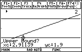
Select that upper bound for the intersection point by pressing
Any point to the right of the point of intersection will work.

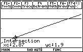
The x-coordinate of the point of intersection is 2.87.

Instead of using the arrow keys to select lower and upper bounds, one can just type in appropriate coordinates if they are known.

Finding the Second Point of Intersection

Now find the point where the graph of the function intersects the upper horizontal line, y3 = 2.1.

Select Intersection from the Math menu by pressing
Select the function as the first curve by pressing
Move the cursor to the top line by pressing

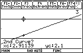
Select y3 as the second curve by pressing
Move the cursor until it is just to the left of the intersection point

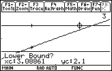
Select the lower bound by pressing
Move the cursor until it is just to the right of the intersection

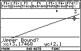
Select the upper bound by pressing

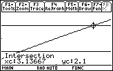
The x-coordinate of this intersection point is approximately 3.13667.

You can conclude that if x is between 2.87 and 3.13666, then y will be within 0.1 of 2. But that was not the original question.

The original question was

It looks like there are two different answers. The left value of 2.87 is within 0.13 of 3. The right value of 3.13666 is within 0.13667 of 3.

4.1.1 Which value of x, 0.13 or 0.13666, will ensure that y is within 0.1 of 2? Click here for the answer.

Smaller Tolerances

4.1.2 For f(x) = , how close should x be to 3 so that y is within 0.01 of 2? Click here for the answer.

< Back | Next >