The Data

The simulation of the spread of a rumor was created by randomly selecting one student to know the rumor on Day 1. On the second day, the initial student then randomly selected a student to tell by using the randInt command. On subsequent days, each student who knew the rumor used the randInt command to select a student to tell. The number of people who know the rumor each day is shown below.

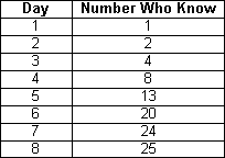
A scatter plot provides a better way to illustrate the data. To do that, the data must be entered into lists in the Stat/List editor.

Creating Data Lists

• Open the Stat/List editor by pressing and selecting 1:Edit.
• Enter the "Day" values in L1 and the "Number Who Know" in L2.

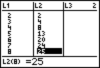
Create a Scatter Plot

Define a scatter plot of the data using squares for the Mark type and display the scatter plot in a ZoomStat window.

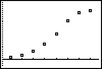
When the data points have a shape like this, it is reasonable to try to find a logistic regression equation to fit the data.

The Logistic Regression Equation

A logistic function models a growth situation that has limited future growth due to a fixed area, food supply, or other factors. Each logistic graph has the same general shape as the data shown above and represents a function of the form

where a, b, and c are constants and e 2.71828. The value of c is the upper limit of the size of y and y = c is a

A line y = c is a horizontal asymptote for the graph of a function if the y-values approach c as the x-values approach positive or negative infinity.

horizontal asymptote of the curve.

Generating the Logistic Regression Equation

The TI-83 can generate a logistic regression equation that best fits the data.

• Return to the Home screen by pressing [QUIT].
• Open the STAT Calc menu by pressing .
• Scroll down to B:Logistic by pressing .

• Paste the Logistic command to the Home screen by pressing .
• Complete the command Logistic L₁, L₂, Y₁ by adding L₁, L₂, and Y₁.
  L₁ and L₂ are above and , and Y₁ is found in the Function submenu in the VARS Y-VARS submenu.

• Execute the command by pressing .

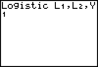
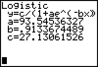
The form of the logistic regression equation is , as shown at the top of the screen, and the values for the coefficients a, b, and c are shown below the equation. The logistic equation that best fits the data is approximately

Graph the Regression Equation

The logistic regression equation is stored in Y₁. Determine how well the graph of the equation fits the scatter plot.

• Display the graph screen by pressing .

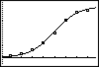
5.2.1 Use the logistic regression equation to estimate the number of people who knew the rumor on the fifth day and compare the estimate to the actual number given in the data. Click here for the answer.