Exponential functions are used in a wide variety of real-world problems. In this lesson you will use transformed exponential functions to model compound interest and radioactive decay and then illustrate the product rule of logarithms graphically.
A Basic Exponential Function
The function y = bx, for b > 0 and b
![]() 1, is called an exponential function. (The possible values for the base, b, are restricted to ensure that the function is well behaved.)
1, is called an exponential function. (The possible values for the base, b, are restricted to ensure that the function is well behaved.)
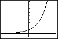
If b > 1, the equation describes exponential growth.
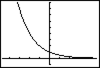
If 0 < b < 1, the equation describes exponential decay.
The basic exponential growth and decay graphs are shown below. In both cases y = bx but the graphs differ depending on the value of b: 0 < b < 1 or b > 1.
|
|
| Exponential Growth b > 1 | Exponential Decay 0 < b < 1 |
Both graphs are asymptotic to the x-axis. The growth graph approaches the x-axis when x is a negative number large in absolute value, and the decay graph approaches the x-axis when x is a large positive number. In each case we say that the graph has a horizontal asymptote of y = 0.
A General Exponential Function
A general exponential function has the form y = a · bx, where b > 0, b
![]() 1, and a is any real number. The effects of transformations that were discussed in Lessons 3.1 and 3.2 hold for any function and apply to the general exponential function.
1, and a is any real number. The effects of transformations that were discussed in Lessons 3.1 and 3.2 hold for any function and apply to the general exponential function.
3.3.1 Describe how the value of a in y = a · bx transforms the graph of y = bx by discussing the associated transformations for the three cases 0 < | a | < 1, | a | > 1, and a < 0. Click here for the answer.
A Compound Interest Problem
If an initial investment of $1000 is compounded annually at an interest rate of 6%, the future value of the investment is given by the exponential growth function
In this equation x is the number of years of the investment and y is the future value of the investment.
- Enter the equation y = 1000 · 1.06 x in the Y= editor.
- Display the table of values associated with y = 1000 · 1.06 x
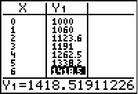
3.3.2 What is the value of the investment after 6 years?
Click here for the answer.
Graphing the Compound Interest Problem
Display a graphical representation for the compound interest problem.
- Graph the equation of y = 1000 · 1.06 x in a [0, 15, 1] x [0, 2500, 500] window.
-
Trace to x = 6 by pressing


 .
.
Note that when tracing in this window, the left and right arrow keys will not display the values when x is exactly 6.
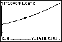
Notice that b = 1.06, which is greater than 1, indicating a growth function, and that a = 1000 indicates that the basic graph of y = 1.06x is stretched vertically by a factor of 1000.
Doubling Time
We are often interested in the time it will take for the investment to double. If the initial investment was $1000, the doubled value will be $2000 and the length of time needed for the investment to double can be found by solving the equation
Find an approximate solution by viewing the table of values for the function y = 1000(1.06) x and determining x when y = 2000.
- Display the table of values by pressing [TABLE] and scroll down to find the x-value that gives the y-value near 2000.
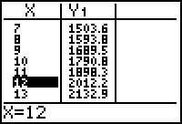
As shown in the table, it will take between 11 and 12 years to double the investment of $1000.
Equivalent Equations
The solution of the equation may be also found by subtracting 2000 from both sides of 2000 = 1000(1.06) x to get an equivalent equation 0 = 1000(1.06)x - 2000, which has the same solution as the original equation.
The screen below shows the graphs of Y1 = 1000(1.06) x and Y2 = 1000(1.06) x - 2000 in a [0, 20, 1] x [-1000, 3000, 500] window. The dotted line is added by graphing Y3=2000 in "dotted line" style and setting Xres equal to 2.
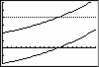
Notice that the x-value that produces the y-value of 2000 in the upper graph is the same x-value that produces the zero in the lower graph. That is, 0 = 1000 · 1.06 x – 2000 has the same solution as 2000 = 1000(1.06) x.
Solving the Doubling Equation Graphically
The right-hand side of y = 1000(1.06) x – 2000 is the exponential function y = 1000(1.06) x that has been shifted downward 2000 units. The zero of the transformed function y = 1000 · 1.06 x – 2000 is the doubling time.
3.3.3 Graph the function y = 1000(1.06) x – 2000 in a [0, 15, 1] x [-2500, 2500, 500] window and use the Zero feature in the Graph screen's CALC menu to find the doubling time. Click here for the answer.
Note that the original equation, 2000 = 1000*1.06x can also be solved by graphing Y1=1000*1.06^x and Y3=2000 and then simply using "intersect" from the CALCULATE menu.
Radioactive Decay
Radioactive dating is often used to determine the age of once-living organisms. The amount of a radioactive substance in a living organism is constant but after it dies the amount of the radioactive substance begins to decay.
A Half-Life Equation
The time it takes for the substance to decay so that half the original amount remains is called its half-life and it is often used to write an equation that will model the amount of the substance present at any given time.
Suppose the half-life of a certain radioactive substance is 30 days. If there are 10 grams present initially, how much will be left after 50 days?
The equation for the amount of radioactive substance, y, remaining after x days is
The equation is equivalent to

Because
![]() may be approximated by y = 10(0.97716) x.
may be approximated by y = 10(0.97716) x.
These equations are equivalent exponential decay functions.
3.3.4 Graph the function y = 10(0.97716) x in a [0, 150, 10] x [-1, 11, 1] window and determine how much is left after 50 days. Click here for the answer.
Solving The Half-Life Equation Graphically
Determine when there will be 1 gram remaining by solving the equation
Subtract 1 from both sides to obtain an equivalent equation whose zero is the solution of the original equation.
The right-hand side of this equation is a transformed exponential decay function. The zero of this transformed function is the time when 1 gram remains.
3.3.5 Graph y = 10(0.97716) x - 1 in a [0, 150, 10] x [-5, 11, 1] window and use the Zero feature in the Graph screen's CALC menu to determine when there will be 1 gram remaining. Click here for the answer.
The Logarithmic Function
The inverse of the exponential function y = bx is the logarithmic function y = logbx. The graphs of the exponential and logarithmic functions are reflections of each other across the line y = x.
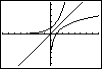
The Exponential and logarithmic functions when b > 1.
Notice that the exponential function's graph has a horizontal asymptote of y = 0 and the logarithmic function's graph has a vertical asymptote of x = 0.
Common Logarithms
When b = 10 the logarithm is called a common logarithm. Usually common logarithms are written as y = log(x) without showing the base b. The common logarithm key,
![]() , on your TI-83 is in the first column.
, on your TI-83 is in the first column.
The Product Rule for Logarithms
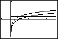
You may illustrate the product rule for logarithms by displaying the graphs of y = log x and y = log 2x.
- Set Y1 = log(x) and Y2 = log(2x).
- Graph the functions in a [-1, 5, 1] x [-2, 2, 1] window.
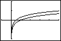
3.3.6 What type of transformation of Y1 = log(x) appears to produce the graph of Y2 = log(2x)? Click here for the answer.
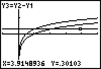
Confirming a Constant Difference
Confirm that the two functions differ by a constant by graphing their difference.
- Set Y3 = Y2 – Y1 in the Y= editor and graph.
Y1 and Y2 are in the VARS Y-VARS Function menu.
3.3.7 Describe how this graph supports the answer to the previous question. Click here for the answer.
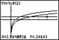
Verifying the Value of the Constant Difference
Verify that the constant difference between the two functions is log(2).
- Set Y4 = log(2) in the Y= editor.
- Display the graphs and select Trace.
- Use the up and down arrow keys to move the Trace cursor between the graphs of Y3 and Y4.
You should see that both functions are displayed, as indicated by the text in the upper left part of the screen, and that they produce the same x and y values, as shown at the bottom of the screen.
|
|
| Graphical evidence that | Y3 and Y4 are the same graph |
The screens above are evidence that the value of the constant C in the answer to 3.3.7 is log(2), and that
The Product Rule for Logarithms
The preceding discussion illustrates the product rule for logarithms:
Explore the effect of multiplying the argument of the logarithm by other values, such as 3, 4, and 5, and graphing y = log(3x), y = log(4x), and y = log(5x).
3.3.8 Based on your results, what is the general product rule for logarithms? Click here for the answer.