In this lesson you will enter data, create a scatter plot of the data, find the regression line that best fits the data, and display the regression line along with the scatter plot.
The Car-Value Example
To illustrate the procedure for creating a scatter plot of a data set and the regression equation that best models the data, the relationship between a car's age and its value will be explored. The following example will guide you to
- illustrate data for a car's value versus its age by creating a scatter plot, and
- find and display a linear equation that best fits the data by using linear regression.
Clearing the Lists
Before a scatter plot can be displayed or a regression equation can be created, the data must be entered into lists in the STAT List editor.
-
Open the STAT EDIT menu by pressing
 .
.
- Open the List editor by selecting 1:Edit.
We want the List Editor to contain the lists L1-L6. If they aren't there, you need to reset the list names in the editor using the following Tech Tip.
|
|||
|
|
|||
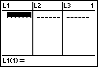
If the list L1 is not empty,
-
Move the cursor to the top of the column until the heading "L1" is highlighted (by using the up arrow key) then press

 .
.
If other lists are not empty,
-
Move the cursor to those lists with
 or
or
 and clear the lists as before.
Creating the Data Lists
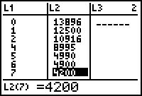
The following values (selling prices) for different ages of a particular model of car were taken from the classified ads of a newspaper. Enter the data into the lists L1 and L2 by following the directions below. The ages will be entered in the list L1 and the corresponding prices will be entered in the list L2.
| Age (yrs) | 0 | 1 | 2 | 4 | 5 | 6 | 7 |
| Price | $13,896 | $12,500 | $10,916 | $8995 | $4990 | $4900 | $4200 |
-
Position the cursor in the top row of L1 (but below the heading "L1") and enter the data for "Age". Press
 after each value to move to the next row.
Move the cursor to L2 with the right arrow key
![]() and enter the values for "Price".
and enter the values for "Price".
Do not use a comma for the large values.
|
|||
|
|
|||
Displaying a Scatter Plot of the Data
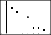
You can illustrate the data with a scatter plot displayed on the Graph screen. The process entails
- defining the plot in the STAT PLOT editor,
- setting the Viewing Window values, and
- displaying the scatter plot.
Defining the Plot
-
Press
 [STAT PLOT] to open the STAT PLOTS menu.
[STAT PLOT] is above the key.
key.
-
Open the STAT PLOT editor for Plot1 by pressing
 .
.
-
Move the cursor to "On" and select it by pressing
 .
.
-
Move the cursor to the line labeled "Type".
The first icon should be blinking. This icon represents a scatter plot. -
Select the scatter plot type and press
 .
.
-
Move the cursor to the line labeled "Xlist" and press
 [L1] to enter L1 as the independent (or input) variable list.
[L1] is above . This will result in having the values from L1, or the ages, plotted along the x-axis.
-
Move the cursor to the line labeled "Ylist" and press
 [L2] to enter L2 as the dependent (or output) variable list.
[L2] is above . This will result in having the values from L2, or the price, plotted along the y-axis.
-
Move the cursor to the line labeled "Mark" and press
 to select the first icon.
This is the mark that will be used for each point in the scatter plot.
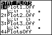
Define the scatter plot in Plot1. Details of the procedure are outlined below.
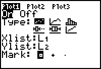
Plot1 should now be defined as shown above.
Set Up the Viewing Window
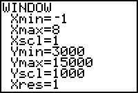
By looking at the data, an appropriate Viewing window for the scatter plot is [-1, 8, 1] x [3000, 15000, 1000].
-
Press
 and enter the values.
Display the Scatter Plot
-
Display the scatter plot by pressing
 .
.
|
|||
|
|
|||
The Linear Regression Equation
The TI-83 has a feature that can be used to find the line that best fits the data. Such a line is called the "regression line" or "line of best fit." The following procedure
- creates the regression line for the data in lists L1 and L2,
- stores the equation in the Y= editor and
- displays the graph of the line with the scatter plot on the Graph screen.
-
Return to and clear the Home screen by pressing
 [QUIT]
 .
.
-
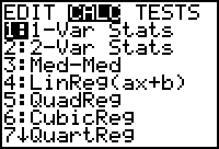
Open the STAT CALC menu by pressing

 .
.
-
Select 4:LinReg(ax+b) by pressing
 .
.
This will paste the command LinReg(ax+b) to the Home screen.
You need to identify which list contains the x-values, which list contains the y-values, and where you would like to store the regression equation.
|
|||
|
|
|||
-
Specify the X-list values by pressing
 [L1], which is above
 .
.
-
Insert a comma between the list names by pressing
 .
.
-
Specify the Y-list values by pressing
 [L2], which is above
 .
.
-
Insert a comma after the Y-list name by pressing
 .
.
-
Select Y1 to hold the linear regression equation using the
 menus.
-
Press
 to execute this command.
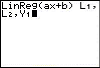
The equation is generated, displayed on the Home screen, and stored in Y1 in the Y= editor.
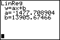
Home Screen
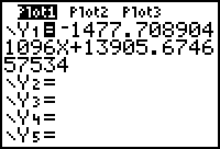
The Regression Equation in the Y= Editor
The linear equation that best fits the data is approximately
where x is the age of the car and y is its value.
-
Press
 to display the graph of the regression equation with the scatter plot.
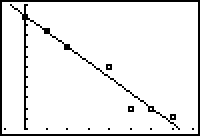
|
|||
|
|
|||
Med-Med
The Med-Med (median-median) feature in the STAT CALC menu fits the model equation y = ax + b to the data using the median-median line technique instead of the least-squares line of best fit technique used by linear regression. Med-Med displays values for a (slope) and b (y-intercept). The syntax for the Med-Med command is the same as the syntax for the LinReg(ax+b) command.
2.2.1 Perform Med-Med on the car-value data in this lesson and compare the resultant equation with the equation found using LinReg(ax+b), y = -1478x + 13,906. Click here for the answer.