Module 3 contained an experiment that simulated the spread of a disease through a small population. In this lesson you will revisit the data used to model the spread of a disease and solve the related differential equation.

Modeling the Data

The following data from a simulation gives the cumulative number of infected people as a disease spreads through a population of 25 people.

Day	Number Infected
1	1
2	2
3	4
4	8
5	13
6	20
7	24
8	25

• Set Graph mode to Function
• Enter the data in your Stats/List Editor and create a scatter plot

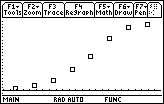
The shape of this scatter plot is called a logistic curve. The differential equation that describes the rate at which the disease spreads is

y' = k * y * (M – y)

where y is the number of infected people, t is time measured in days, M is the maximum possible number of infected people and k is a constant. For this simulation, M is 25.

You will use the "guess and check" method to find an approximation for k that fits the data by graphing solutions to the differential equations for different values of k . Use an initial guess of 0.05 for k.

• Perform NewProb
• Select Differential Equation graphing mode on your TI-89
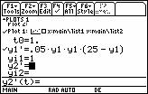
• Store the differential equation y1' = 0.05 * y1 * (25 – y1) into y1'

Remember to include the multiplication sign before the parenthesis.

• Enter the initial conditions t0 = 1 and yi1 = 1

• Open the Format menu by pressing
• Move the cursor to the line labeled "Fields"
• Turn the slope field off by pressing
• Save your selection by pressing
• Display the graph of the data and the solution to the differential equation by selecting "9:ZoomData" from the F2:Zoom menu

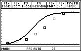
20.1.1 Modify k until the graph of the solution to the differential equation approximates the scatter plot.
Click here for the answer.

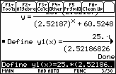
After you have found the value of k, use deSolve to find the solution to the differential equation.

• deSolve(y' = 0.037*y*(25 - y) and y(1)=1,x,y)

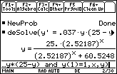
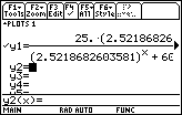
• Change your TI-89 to Function graphing mode and store the solution to the differential equation in y1(x)

Storing Functions into the Y=Editor from the Home Screen Paste the equation for y from the History Area to the Edit Line Notice that the TI-89 displays a limited number of significant digits when results are displayed in the History area. This is determined by the "Display Digits" setting on the mode screen. But the TI-89 always stores 14 significant digits for results, and they are all displayed in the Edit Line and the Y= editor. Replace the "y" on the left side of the equation with "Define y1(x)" Press Check the Y= Editor to see that this procedure placed the logistic equation in y1

• Display the graph of the solution to the logistic differential equation together with the scatter plot by pressing

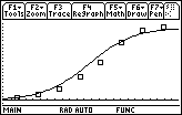
This graph was generated in the answer to 20.1.1 using the numerical Differential Equation solver in Differential Equation graphing mode that does not result in a formula for the solution. This time we generated the graph by solving the Differential Equation symbolically and graphed the solution in Function Mode.