In Lesson 15.1 you used right-hand rectangles to find the area of the region bounded by the graph of f(x) = x², the vertical line x = 1, and the x-axis. In this lesson you will use left-hand Riemann sums to find the same area.

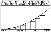
The sum of the areas of the rectangles shown above is called a left-hand Riemann sum because the left-hand corner of each rectangle is on the curve.

Defining the Left-hand Sum Function

A function similar to the one defined in Lesson 15.1 can be used to find the sum of the areas of the rectangles under the curve defined by f(x) between the vertical lines x = a and x = b and above the x-axis using left-hand rectangles. Modifying the command that defined rrs can create the new function.

• Paste the command you used to define rrs from the History Area to the Edit Line
• Change rrs to lrs

The first left-hand x-coordinate is found by letting k = 0 and the last left-hand x-coordinate is found by letting k = n – 1. This replaces the first right-hand x-coordinate found by letting k = 1 and the last right-hand x-coordinate found by letting k = n.

• Change the initial value and ending value of the sum function from "1, n" to "0, n –1"
• Define

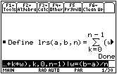
The function f(x) = x² should still be defined from Lesson 15.1. The following exploration uses the same procedure used to find the right-hand Riemann sum using four rectangles, except this time the left-hand function lrs will be used to approximate the area under the curve.

• Select Approximate Mode
• Enter lrs(0,1,4)

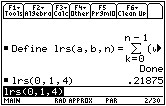
• Evaluate the left-hand Riemann sum for 10, 50 and 100 rectangles.

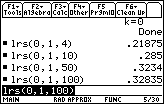
The areas found using left-hand rectangles appear to converge to the same limit as the areas found using right-hand rectangles, .

• Set Exact/Approx back to Auto Mode

15.2.1 Evaluate limit(lrs(0,1,n),n, ) and interpret the result.

Click here for the answer.

When the number of rectangles approaches infinity, the left-hand function lrs has the same limit as the right-hand function rrs. That is, the area under the curve can be found by using either right or left Reimann sum limits as the number of rectangles approaches because they produce the same result. This is true in general for continuous functions, and in fact, any x-value in each subinterval on the x-axis can be used to determine the height of the corresponding rectangle.

The area Program

A program can be used to illustrate the rectangles that approximate the area under a curve. The program area draws the rectangles associated with left, right and

Midpoint Riemann sums are obtained by using the midpoint of each subinterval on the x-axis to determine the height of the corresponding rectangle.

midpoint Riemann sums under a curve and displays the sum of the areas associated with each type. It was used to create the pictures of Riemann sum rectangles earlier in this lesson and in Lesson 15.1, and with the program you can create similar visual representations.

Downloading the area Program

• Click here to download the program area
• Choose to save the file
• Save the file on your local hard disk in a folder that you can access later

Transferring the Program to the TI-89

Click here to get information about how to obtain the needed cable and to review the procedure to transfer the program from your computer to your calculator.

• Transfer the program area to your TI-89 calculator
• Clear the Home Screen

Using the area Program

The following procedure illustrates the approximate area of the region bounded by the graph of f(x) = x², the vertical line x = 1, and the x-axis by drawing rectangles associated with the left, right and midpoint Riemann sums.

The function x² should be stored in y1 in the Y= Editor.

• Enter the [0, 1] x [0,1] viewing window and return to the Home screen
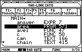
• Display the list of variables in the MAIN folder by pressing

The MAIN folder may be expanded by pressing , if necessary.

• Highlight area in the listing

• Paste the area program name to the Edit Line of the Home Screen by pressing
• Provide the closing parenthesis by pressing

The parentheses should be empty.

• Run the program by pressing

You should see a prompt for the value of a, the left side of the region.

• Enter 0 and press

Now you should see a prompt for the value of b, the right side of the region.

• Enter 1 and press

Next you see a prompt for the number of subintervals, i.e., the number of rectangles.

• Enter 10

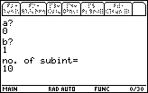
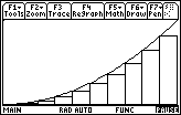
The graph of f(x) = x² with the left-hand rectangles will be displayed when you press . The pause indicator should appear in the lower right-hand corner of the screen.

Viewing the Next Screens

Subsequent screens of the program display the areas obtained by using all three methods and illustrations of the right and midpoint Riemann sums.

• Display the left Riemann sum by pressing
• Display the right-hand rectangles by pressing

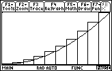
• Move through the remaining screens by pressing repeatedly

You should see the right Riemann sum, the illustration of midpoint rectangles, and finally the midpoint Riemann sum.

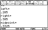
The sums of the ten rectangles used to evaluate the area of the region using left, right, and midpoint rectangles are 0.285, 0.385, and 0.3325, respectively.

• Return to the Home screen by pressing

15.2.2 Use the area program to illustrate the area under f(x) = 2x + 1 between x = 0 and x = 3 using 6 rectangles, and find the approximate area using left, right, and midpoint rectangles.

Click here for the answer.