Module 5 contained an experiment that simulated the spread of a rumor through a small population. In this lesson you will revisit that data and solve the related differential equation.
Modeling the Data
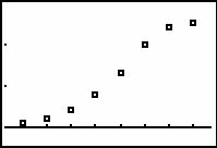
The following data from a simulation gives the cumulative number of people who know a rumor as it spreads through a population of 25 people.
| Day | Number Who Knew |
| 1 | 1 |
| 2 | 2 |
| 3 | 4 |
| 4 | 8 |
| 5 | 13 |
| 6 | 20 |
| 7 | 24 |
| 8 | 25 |
-
Enter the data in your Stats/List Editor, set up Plot1, and create a scatter plot by pressing
 and selecting 9:ZoomStat.

[0.3, 8.7, 1] x [-3.08, 29.08, 10]
The shape of this scatter plot is called a logistic curve. The differential equation that describes the rate at which the rumor spreads is
where y is the number of people who know the rumor at time t. t is time measured in days, M is the maximum possible number of people who can know the rumor, and k is a constant. For this simulation, M is 25.
You will use the "Guess and Check" method to find an approximation for k that fits the data by graphing solutions to the differential equation for different values of k. Use an initial guess of 0.05 for k.
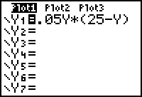
- Set Y1 = 0.05Y*(25-Y).
- If necessary, click here to download EULERG to your computer then reinstall the program on your calculator.
- Run program EULERG.
- Enter the initial conditions Initial X = 1 and Y(Initial X) = 1.
- Enter a step size of 0.05.


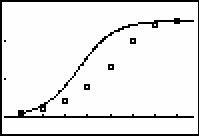
The solution to the differential equation with k = 0.05 has the correct general shape but does not fit the data very well.
22.1.1 Modify the value of k in Y1 and run program EULERG again to get a better fit to the scatter plot. Continue to modify k and run EULERG until the graph of the solution to the differential equation approximates the scatter plot well. What value of k seems to work best?
Click here for the answer.