In Lesson 1.2 you defined the function f(x) = 2x² – 5x – 3 and found its roots symbolically. In Lesson 1.3 you graphed the function and found its roots graphically. In this lesson you will represent the function numerically with a table and use the table to find the roots.

Creating a Table of Function Values

To make a table of values for a function, you need to enter the function in the Y= Editor. You should have already done this in Lesson 1.3.

• Make sure f(x) is still stored in y1 by pressing [Y=] to view the Y= Editor

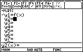
Displaying the Table Setup Dialog Box

Before you view the table, you should set its parameters.

• View the Table parameters, which are displayed in the Table Setup Dialog box, by pressing

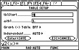
Table Setup Parameters

The value in tblStart will be the first value of x in the table.

• Enter -1 next to tblStart
• Save the value by pressing

The value in tbl determines how much x increases when moving from one row to the next in the table. This value should be 1. Make sure the other settings match the figure shown below, and then press to save all the table parameter values. This should return you to the Y= Editor.

Saving Table Setup Parameters When editing values in the Table Setup Dialog box, you will need to press after each value and then press to exit the Table Setup Dialog box. If you try to exit the dialog box by pressing or by pressing [TABLE] to jump to the table, the changes you made will not be saved, and you will not see the values you expect in the table.

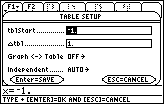
• View the table of values of f(x) = 2x² – 5x – 3 for x = -1, 0, 1, 2, and 3 by pressing [TABLE].
  [TABLE] is above .

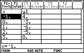
Finding Roots from a Table

The table provides numerical evidence for two roots. One root must exist between x = -1 and x = 0 because the corresponding values in y1 change sign and the function is continuous, i.e., it has no breaks. The other root is x = 3 because the corresponding value of y1 is 0.

You can get a better approximation of the root between -1 and 0 by changing tbl to 0.1.

• Return to the Table Setup Dialog Box by pressing [TblSet] and change the value of tbl to 0.1

You can move up and down within the dialog box with the cursor movement keys .

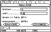
Change the value of tbl to 0.1

• After you change the value of tbl, press twice, once to save the value in tbl and once to exit the Table Setup dialog box
• If you were viewing the table before you changed the Table Setup parameters, exiting the Table Setup Dialog box will return you immediately to the Table screen with the new table. Otherwise, press [TABLE] to view the new Table.
• Scroll down with until you see the root at x = -0.5.

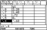
Scroll to see the root at –.5

This method of expanding the table between x = -1 and x = 0 is called table zoom.

1.4.1 What root is shown in the table above? Click here for the answer.