% t v
% t displays a menu with the following options:
| • | 1-Var Stats analyzes statistical data from 1 data set with 1 measured variable, x. |
| • | 2-Var Stats analyzes paired data from 2 data sets with 2 measured variables—x, the independent variable, and y, the dependent variable. |
| • | StatVars displays a secondary menu of statistical variables. The StatVars menu only appears after you have calculated 1-Var or 2-Var stats. Use $ and # to locate the desired variable, and press < to select it. |
|
Variables |
Definition |
|
n |
Number of x or (x,y) data points. |
|
Ï or Ð |
Mean of all x or y values. |
|
Sx or Sy |
Sample standard deviation of x or y. |
|
Îx or Îy |
Population standard deviation of x or y. |
|
Gx or Gy |
Sum of all x or y values. |
|
Gx2 or Gy2 |
Sum of all x2 or y2 values. |
|
Gxy |
Sum of (x…y) for all xy pairs. |
|
a |
Linear regression slope. |
|
b |
Linear regression y-intercept. |
|
r |
Correlation coefficient. |
|
xÅ (2-Var) |
Uses a and b to calculate predicted x value when you input a y value. |
|
yÅ (2-Var) |
Uses a and b to calculate predicted y value when you input an x value. |
|
MinX |
Minimum of x values. |
|
Q1 (1-Var) |
Median of the elements between MinX and Med (1st quartile). |
|
Med |
Median of all data points. |
|
Q3 (1-Var) |
Median of the elements between Med and MaxX (3rd quartile). |
|
MaxX |
Maximum of x values. |
To define statistical data points:
| 1. | Enter data in L1, L2, or L3. (See Data editor.) |
Note: Non-integer frequency elements are valid. This is useful when entering frequencies expressed as percentages or parts that add up to 1. However, the sample standard deviation, Sx, is undefined for non-integer frequencies, and Sx = Error is displayed for that value. All other statistics are displayed.
| 2. | Press % t. Select 1-Var or 2-Var and press <. |
| 3. | Select L1, L2, or L3, and the frequency. |
| 4. | Press < to display the menu of variables. |
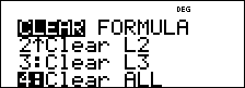
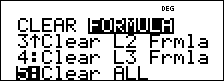
| 5. | To clear data, press v v, select a list to clear, and press <. |
Examples
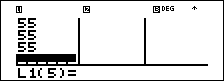
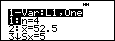
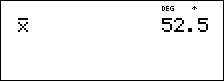
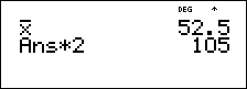
1-Var: Find the mean of {45, 55, 55, 55}
|
Clear all data |
v v $ $ $ |
|
|
Data |
< 45 $ 55 $ 55 $ 55 < |
|
|
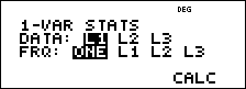
Stat |
% t 1 |
|
|
|
$ $ |
|
|
|
< |
|
|
Stat Var |
2 < |
|
|
|
V 2 < |
|


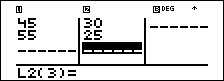
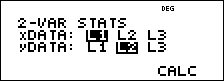
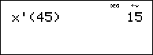
2-Var: Data: (45,30); (55,25). Find: xÅ(45)
|
Clear all data |
v v $ $ $ |
|
|
Data |
< 45 $ 55 $ " 30 $ 25 $ |
|
|
Stat |
% t 2 (Your screen may not show |
|
|
|
$ $ |
|
|
|
< % Q % t 3 # # # # # # |
|
|
|
< 45 E < |
|


³ Problem
For his last four tests, Anthony obtained the following scores. Tests 2 and 4 were given a weight of 0.5, and tests 1 and 3 were given a weight of 1.
|
Test No. |
1 |
2 |
3 |
4 |
|
Score |
12 |
13 |
10 |
11 |
|
Coefficient |
1 |
0.5 |
1 |
0.5 |
| 1. | Find Anthony’s average grade (weighted average). |
| 2. | What does the value of n given by the calculator represent? What does the value of Gx given by the calculator represent? |
Reminder: The weighed average is

| 3. | The teacher gave Anthony 4 more points on test 4 due to a grading error. Find Anthony’s new average grade. |
|
v v 4 v " 5 |
|
|
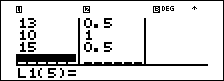
12 $ 13 $ 10 $ 11 $ " 1 $ .5 $ 1 $ .5 $ |
|
|
% t 1 (Your screen may not show |
|
|
$ " " < |
|
|
< |
|
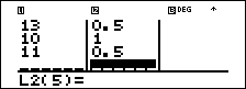

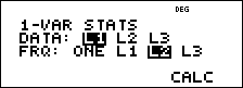
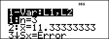
Anthony has an average (Ï) of 11.33 (to the nearest hundredth).
On the calculator, n represents the total sum of the weights.
n = 1 + 0.5 + 1 + 0.5
Gx represents the weighted sum of his scores.
(12)(1) + (13)(0.5) + (10)(1) + (11)(0.5) = 34
Change Anthony’s last score from 11 to 15.
|
v $ $ $ 15 $ |
|
|
% t 1 $ $ < |
|
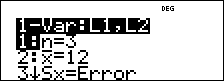
If the teacher adds 4 points to Test 4, Anthony’s average grade is 12.
³ Problem
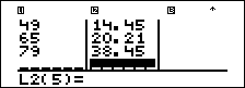
The table below gives the results of a braking test.
|
Test No. |
1 |
2 |
3 |
4 |
|
Speed (kph) |
33 |
49 |
65 |
79 |
|
Braking distance (m) |
5.30 |
14.45 |
20.21 |
38.45 |
Use the relationship between speed and braking distance to estimate the braking distance required for a vehicle traveling at 55 kph.
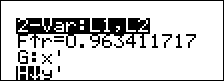
A hand-drawn scatter plot of these data points suggest a linear relationship. The TI‑30XS MultiView™ calculator uses the least squares method to find the line of best fit, y'=ax'+b, for data entered in lists.
|
v v 4 |
|
|
33 $ 49 $ 65 $ 79 $ " 5.3 $ 14.45 $ 20.21 $ 38.45 $ |
|
|
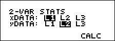
% t 2 |
|
|
$ $ |
|
|
< |
|
|
Press $ to view a and b. |
|


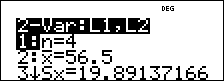
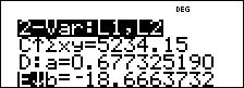
This line of best fit, y'=0.67732519x'-18.66637321 models the linear trend of the data.
|
Press $ until y' is highlighted. |
|
|
< 55 E < |
|
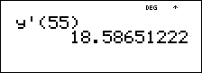
The linear model gives an estimated braking distance of 18.59 meters for a vehicle traveling at 55 kph.