v % u
v lets you enter and edit the data lists. (See Data Editor section.)
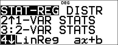
% u displays the STAT-REG menu, which has the following options.
Notes:
| • | Regressions store the regression information, along with the 2-Var statistics for the data, in StatVars (menu item 1). |
| • | A regression can be stored to either f(x) or g(x). The regression coefficients display in full precision. |
Important note about results: Many of the regression equations share the same variables a, b, c, and d. If you perform any regression calculation, the regression calculation and the 2-Var statistics for that data are stored in the StatVars menu until the next statistics or regression calculation. The results must be interpreted based on which type of statistics or regression calculation was last performed. To help you interpret correctly, the title bar reminds you of which calculation was last performed.
|
1:StatVars |
Displays a secondary menu of the last computed statistical result variables. Use $ and # to locate the desired variable, and press < to select it. If you select this option before calculating 1-Var stats, 2-Var stats, or any of the regressions, a reminder appears. |
|
2:1-VAR STATS |
Analyzes statistical data from 1 data set with 1 measured variable, x. Frequency data may be included. |
|
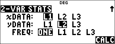
3:2-VAR STATS |
Analyzes paired data from 2 data sets with 2 measured variables—x, the independent variable, and y, the dependent variable. Frequency data may be included. Note: 2-Var Stats also computes a linear regression and populates the linear regression results. It displays values for a (slope) and b (y-intercept); it also displays values for r2 and r. |
|
4:LinReg ax+b |
Fits the model equation y=ax+b to the data using a least-squares fit for at least two data points. It displays values for a (slope) and b (y-intercept); it also displays values for r2 and r. |
|
5:PropReg ax |
Fits the model equation y=ax to the data using using least squares fit for at least one data point. It displays the value for a. Supports data forming a vertical line with the exception of all 0 data. |
|
6:RecipReg a/x+b |
Fits the model equation y=a/x+b to the data using least squares fit on linearized data for at least two data points. It displays values for a and b; it also displays values for r2 and r. |
|
7:QuadraticReg |
Fits the second-degree polynomial y=ax2+bx+c to the data. It displays values for a, b, and c; it also displays a value for R2. For three data points, the equation is a polynomial fit; for four or more, it is a polynomial regression. At least three data points are required. |
|
8:CubicReg |
Fits the third-degree polynomial y=ax3+bx2+cx+d to the data. It displays values for a, b, c, and d; it also displays a value for R2. For four points, the equation is a polynomial fit; for five or more, it is a polynomial regression. At least four points are required. |
|
9:LnReg a+blnx |
Fits the model equation y=a+b ln(x) to the data using a least squares fit and transformed values ln(x) and y. It displays values for a and b; it also displays values for r2 and r. |
|
:PwrReg ax^b |
Fits the model equation y=axb to the data using a least-squares fit and transformed values ln(x) and ln(y). It displays values for a and b; it also displays values for r2 and r. |
|
:ExpReg ab^x |
Fits the model equation y=abx to the data using a least-squares fit and transformed values x and ln(y). It displays values for a and b; it also displays values for r2 and r. |
|
:expReg ae^(bx) |
Fits the model equation y=a e^(bx) to the data using least squares fit on linearized data for at least two data points. It displays values for a and b; it also displays values for r2 and r. |
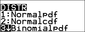
% u " displays the DISTR menu, which has the following distribution functions:
|
1:Normalpdf |
Computes the probability density function (pdf) for the normal distribution at a specified x value. The defaults are mean mu=0 and standard deviation sigma=1. The probability density function (pdf) is:
|
|
2:Normalcdf |
Computes the normal distribution probability between LOWERbnd and UPPERbnd for the specified mean mu and standard deviation sigma. The defaults are mu=0; sigma=1; with LOWERbnd = M1E99 and UPPERbnd = 1E99. Note: M1E99 to 1E99 represents Minfinity to infinity. |
|
3:invNormal |
Computes the inverse cumulative normal distribution function for a given area under the normal distribution curve specified by mean mu and standard deviation sigma. It calculates the x value associated with an area to the left of the x value. 0 { area { 1 must be true. The defaults are area=1, mu=0 and sigma=1. |
|
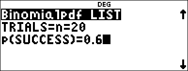
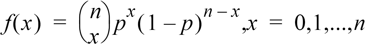
4:Binomialpdf |
Computes a probability at x for the discrete binomial distribution with the specified numtrials and probability of success (p) on each trial. x is a non-negative integer and can be entered with options of SINGLE entry, LIST of entries or ALL (list of probabilities from 0 to numtrials is returned). 0 { p { 1 must be true. The probability density function (pdf) is:
|
|
5:Binomialcdf |
Computes a cumulative probability at x for the discrete binomial distribution with the specified numtrials and probability of success (p) on each trial. x can be non-negative integer and can be entered with options of SINGLE, LIST or ALL (a list of cumulative probabilities is returned.) 0 { p { 1 must be true. |
|
6:Poissonpdf |
Computes a probability at x for the discrete Poisson distribution with the specified mean mu (m), which must be a real number > 0. x can be an non-negative integer (SINGLE) or a list of integers (LIST). The default is mu=1. The probability density function (pdf) is:
|
|
7:Poissoncdf |
Computes a cumulative probability at x for the discrete Poisson distribution with the specified mean mu, which must be a real number > 0. x can be an non-negative integer (SINGLE) or a list of integers (LIST). The default is mu=1. |


Stats Results
|
Variables |
1-Var or 2-Var |
Definition |
|---|---|---|
|
n |
Both |
Number of x or (x,y) data points. |
|
v |
Both |
Mean of all x values. |
|
w |
2-Var |
Mean of all y values. |
|
Sx |
Both |
Sample standard deviation of x. |
|
Sy |
2-Var |
Sample standard deviation of y. |
|
sx |
Both |
Population standard deviation of x. |
|
sy |
2-Var |
Population standard deviation of y. |
|
Gx or Gx2 |
Both |
Sum of all x or x2 values. |
|
Gy or Gy2 |
2-Var |
Sum of all y or y2 values. |
|
Gxy |
2-Var |
Sum of (xQy) for all xy pairs. |
|
a |
2-Var |
Linear regression slope. |
|
b |
2-Var |
Linear regression y-intercept. |
|
r2 or r |
2-Var |
Correlation coefficient. |
|
x¢ |
2-Var |
Uses a and b to calculate predicted x value when you input a y value. |
|
y¢ |
2-Var |
Uses a and b to calculate predicted y value when you input an x value. |
|
minX or maxX |
Both |
Minimum or maximum of x values. |
|
Q1 |
1-Var |
Median of the elements between minX and Med (1st quartile). |
|
Med |
1-Var |
Median of all data points. |
|
Q3 |
1-Var |
Median of the elements between Med and maxX (3rd quartile). |
|
minY or maxY |
2-Var |
Minimum or maximum of y values. |
To define statistical data points:
| 1. | Enter data in L1, L2, or L3. (See Data Editor section.) |
Note: Non-integer frequency elements are valid. This is useful when entering frequencies expressed as percentages or parts that add up to 1. However, the sample standard deviation, Sx, is undefined for non-integer frequencies, and Sx=Error is displayed for that value. All other statistics are displayed.
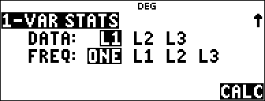
| 2. | Press % u. Select 1-Var or 2-Var and press <. |
| 3. | Select L1, L2, or L3, and the frequency. |
| 4. | Press < to display the menu of variables. |
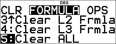
| 5. | To clear data, press v v, select a list to clear, and press <. |
1-Var Example
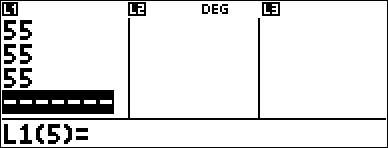
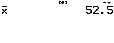
Find the mean of {45,55,55,55}.
|
Clear all data |
v v $ $ $ |
|
|
Data |
< 45 $ 55 $ 55 $ 55 < |
|
|
Stat |
% s % u |
|
|
|
2 (Selects 1-VAR STATS) $ $ |
|
|
|
< |
|
|
Stat Var |
2 < |
|
|
|
V 2 < |
|


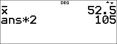
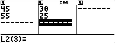
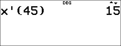
2-Var Example
Data: (45,30); (55,25). Find: x¢(45).
|
Clear all data |
v v $ $ $ |
|
|
Data |
< 45 $ 55 $ " 30 $ 25 $ |
|
|
Stat |
% u |
|
|
|
3 (Selects 2-VAR STATS) $ $ $ |
|
|
StatVars |
< % s % u 1 # # # # # # |
|
|
|
< 45 ) < |
|

Problem
For his last four tests, Anthony obtained the following scores. Tests 2 and 4 were given a weight of 0.5, and tests 1 and 3 were given a weight of 1.
|
Test No. |
1 |
2 |
3 |
4 |
|
Score |
12 |
13 |
10 |
11 |
|
Weight |
1 |
0.5 |
1 |
0.5 |
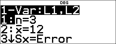
| 1. | Find Anthony’s average grade (weighted average). |
| 2. | What does the value of n given by the calculator represent? What does the value of Gx given by the calculator represent? |
Reminder: The weighted average is

| 3. | The teacher gave Anthony 4 more points on test 4 due to a grading error. Find Anthony’s new average grade. |
|
v v $ $ $ |
|
|
< v " $ $ $ $ |
|
|
< 12 $ 13 $ 10 $ 11 $ " 1 $ .5 $ 1 $ .5 < |
|
|
% u |
|
|
2 $ " " < |
|
|
< |
|


Anthony has an average (v) of 11.33 (to the nearest hundredth).
On the calculator, n represents the total sum of the weights.
n = 1 + 0.5 + 1 + 0.5.
Gx represents the weighted sum of his scores.
(12)(1) + (13)(0.5) + (10)(1) + (11)(0.5) = 34.
Change Anthony’s last score from 11 to 15.
|
v $ $ $ 15 < |
|
|
% u 2 $ " " < < |
|

If the teacher adds 4 points to Test 4, Anthony’s average grade is 12.
Problem
The table below gives the results of a braking test.
|
Test No. |
1 |
2 |
3 |
4 |
|
Speed (kph) |
33 |
49 |
65 |
79 |
|
Braking distance (m) |
5.30 |
14.45 |
20.21 |
38.45 |
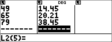
Use the relationship between speed and braking distance to estimate the braking distance required for a vehicle traveling at 55 kph.
A hand-drawn scatter plot of these data points suggest a linear relationship. The calculator uses the least squares method to find the line of best fit, y'=ax'+b, for data entered in lists.
|
v v $ $ $ |
|
|
< 33 $ 49 $ 65 $ 79 $ " 5.3 $ 14.45 $ 20.21 $ 38.45 < |
|
|
% s % u |
|
|
3 (Selects 2-VAR STATS) $ $ $ |
|
|
< |
|
|
Press $ as necessary to view a and b. |
|

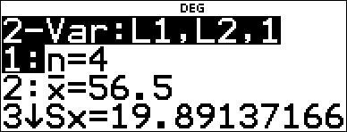
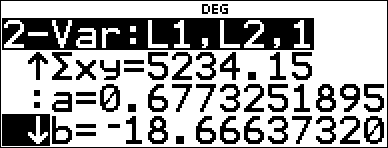
This line of best fit, y'=0.67732519x'N18.66637321 models the linear trend of the data.
|
Press $ until y' is highlighted. |
|
|
< 55 ) < |
|

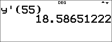
The linear model gives an estimated braking distance of 18.59 meters for a vehicle traveling at 55 kph.
Regression Example 1
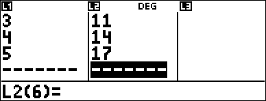
Calculate an ax+b linear regression for the following data: {1,2,3,4,5}; {5,8,11,14,17}.
|
Clear all data |
v v $ $ $ |
|
|
Data |
< 1 $ 2 $ 3 $ 4 $ 5 $ " 5 $ 8 $ 11 $ 14 $ 17 < |
|
|
Regression |
% s % u $ $ $ |
|
|
|
< |
|
|
|
$ $ $ $ < Press $ to examine all the result variables. |
|
Regression Example 2
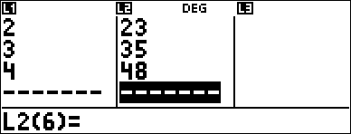
Calculate the exponential regression for the following data:
| • | L1 = {0,1,2,3,4}; L2 = {10,14,23,35,48} |
| • | Find the average value of the data in L2. |
| • | Compare the exponential regression values to L2. |
|
Clear all data |
v v 4 |
|
|
Data |
0 $ 1 $ 2 $ 3 $ 4 $ " 10 $ 14 $ 23 $ 35 $ 48 < |
|
|
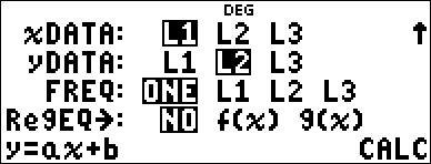
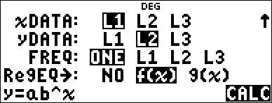
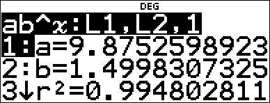
Regression |
% u # # |
|
|
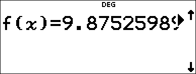
Save the regression equation to f(x) in the I menu. |
< $ $ $ " < |
|
|
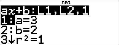
Regression Equation |
< |
|
|
Find the average value (y) of the data in L2 using StatVars. |
% u 1 (Selects StatVars) $ $ $ $ $ $ $ $ |
Notice that the title bar reminds you of your last statistical or regression calculation. |
|
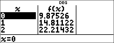
Examine the table of values of the regression equation. |
I 1 |
|
|
|
< $ 0 < 1 < |
|
|
|
< < |
|


Warning: If you now calculate 2-Var Stats on your data, the variables a and b (along with r and r2) will be calculated as a linear regression. Do not recalculate 2-Var Stats after any other regression calculation if you want to preserve your regression coefficients (a, b, c, d) and r values for your particular problem in the StatVars menu.
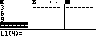
Distribution Example
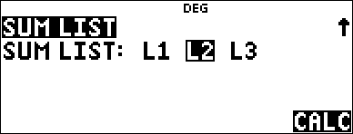
Compute the binomial pdf distribution at x values {3,6,9} with 20 trials and a success probability of 0.6. Enter the x values in list L1, store the results in L2, and then find the sum of the probabilities and store in the variable t.
|
Clear all data |
v v $ $ $ |
|
|
Data |
< 3 $ 6 $ 9 < |
|
|
DISTR |
% u " $ $ $ |
|
|
|
< " |
|
|
|
< 20 $ 0.6 |
|
|
|
< $ $ |
|
|
|
< |
|
|
|
v ! 4 " < |
|
|
|
< " " " " < < |
|