|
Catalog > |
|
|
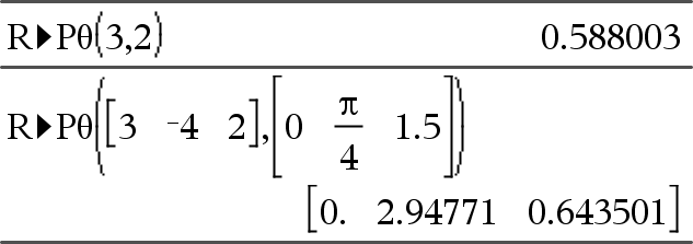
Returns the equivalent θ-coordinate of the Note: The result is returned as a degree, gradian or radian angle, according to the current angle mode setting. Note: You can insert this function from the computer keyboard by typing R@>Ptheta(...). |
In Degree angle mode:
|
|
Catalog > |
|
|
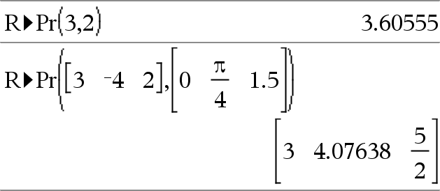
Returns the equivalent r-coordinate of the (x,y) pair arguments. Note: You can insert this function from the computer keyboard by typing R@>Pr(...). |
In Radian angle mode:
|
|
Catalog > |
|
|
Converts the argument to radian angle measure. Note: You can insert this operator from the computer keyboard by typing @>Rad. |
In Degree angle mode:
|
|
Catalog > |
|
|
rand() ⇒ expression rand() returns a random value between 0 and 1. rand(#Trials) returns a list containing #Trials random values between 0 and 1. |
Set the random-number seed.
|
|
Catalog > |
|
|
randBin(n, p) ⇒ expression randBin(n, p) returns a random real number from a specified Binomial distribution. randBin(n, p, #Trials) returns a list containing #Trials random real numbers from a specified Binomial distribution. |
|
|
Catalog > |
|
|
randInt(lowBound,upBound) ⇒ expression randInt(lowBound,upBound) returns a random integer within the range specified by lowBound and upBound integer bounds. randInt(lowBound,upBound ,#Trials) returns a list containing #Trials random integers within the specified range. |
|
|
Catalog > |
|
|
randMat(numRows, numColumns) ⇒ matrix Returns a matrix of integers between -9 and 9 of the specified dimension. Both arguments must simplify to integers. |
Note: The values in this matrix will change each time you press ·. |
|
Catalog > |
|
|
randNorm(μ, σ) ⇒ expression randNorm(μ, σ) returns a decimal number from the specified normal distribution. It could be any real number but will be heavily concentrated in the interval [μ−3•σ, μ+3•σ]. randNorm(μ, σ, #Trials) returns a list containing #Trials decimal numbers from the specified normal distribution. |
|
|
Catalog > |
|
|
randPoly(Var, Order) ⇒ expression Returns a polynomial in Var of the specified Order. The coefficients are random integers in the range −9 through 9. The leading coefficient will not be zero. Order must be 0–99. |
|
|
Catalog > |
|
|
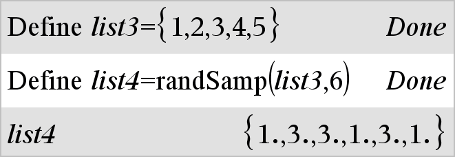
randSamp(List,#Trials[,noRepl]) ⇒ list Returns a list containing a random sample of #Trials trials from List with an option for sample replacement (noRepl=0), or no sample replacement (noRepl=1). The default is with sample replacement. |
|
|
Catalog > |
|
|
RandSeed Number If Number = 0, sets the seeds to the factory defaults for the random-number generator. If Number ≠ 0, it is used to generate two seeds, which are stored in system variables seed1 and seed2. |
|
|
Catalog > |
|
|
real(Value1) ⇒ value Returns the real part of the argument. |
|
|
real(List1) ⇒ list Returns the real parts of all elements. |
|
|
real(Matrix1) ⇒ matrix Returns the real parts of all elements. |
|
|
Catalog > |
|
|
Vector ►Rect Note: You can insert this operator from the computer keyboard by typing @>Rect. Displays Vector in rectangular form [x, y, z]. The vector must be of dimension 2 or 3 and can be a row or a column. Note: ►Rect is a display-format instruction, not a conversion function. You can use it only at the end of an entry line, and it does not update ans. Note: See also ►Polar, here. |
|
|
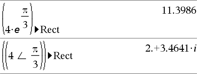
complexValue ►Rect Displays complexValue in rectangular form a+bi. The complexValue can have any complex form. However, an reiθ entry causes an error in Degree angle mode. Note: You must use parentheses for an (r∠θ) polar entry. |
In Radian angle mode:
Note: To type ∠, select it from the symbol list in the Catalog. |
|
Catalog > |
|||||||
|
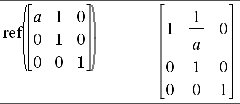
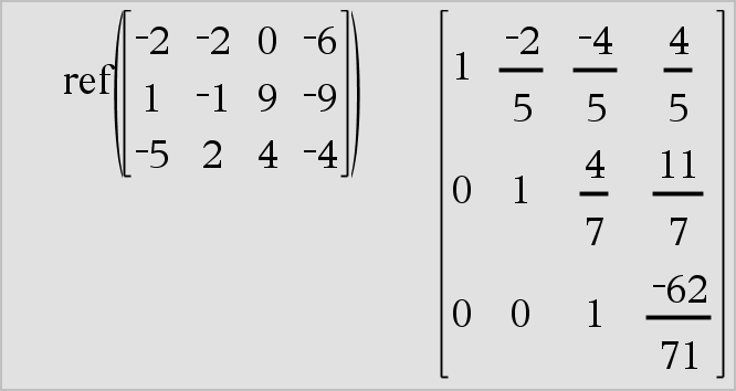
ref(Matrix1[, Tol]) ⇒ matrix Returns the row echelon form of Matrix1. Optionally, any matrix element is treated as zero if its absolute value is less than Tol. This tolerance is used only if the matrix has floating-point entries and does not contain any symbolic variables that have not been assigned a value. Otherwise, Tol is ignored.
Avoid undefined elements in Matrix1. They can lead to unexpected results. For example, if a is undefined in the following expression, a warning message appears and the result is shown as:
The warning appears because the generalized element 1/a would not be valid for a=0. You can avoid this by storing a value to a beforehand or by using the constraint (“|”) operator to substitute a value, as shown in the following example.
Note: See also rref(), here. |
|
|
Catalog > |
|||||||||||
|
RefreshProbeVars Allows you to access sensor data from all connected sensor probes in your TI-Basic program.
|
Example
Note: This can also be used with TI-Innovator™ Hub. |
|
Catalog > |
|
|
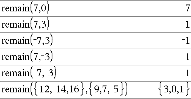
Returns the remainder of the first argument with respect to the second argument as defined by the identities: remain(x,0) x |
|
|
As a consequence, note that remain(−x,y) − remain(x,y). The result is either zero or it has the same sign as the first argument. Note: See also mod(), here. |
|
|
Catalog > |
|||||||||||||||||||
|
Programming command: Pauses the program and displays a dialog box containing the message promptString and an input box for the user’s response. When the user types a response and clicks OK, the contents of the input box are assigned to variable var. If the user clicks Cancel, the program proceeds without accepting any input. The program uses the previous value of var if var was already defined. The optional DispFlag argument can be any expression.
|
Define a program: Define request_demo()=Prgm
Run the program and type a response: request_demo()
Result after selecting OK: Radius: 6/2 |
||||||||||||||||||
|
The optional statusVar argument gives the program a way to determine how the user dismissed the dialog box. Note that statusVar requires the DispFlag argument.
The func() argument allows a program to store the user’s response as a function definition. This syntax operates as if the user executed the command: Define func(arg1, ...argn) = user’s response The program can then use the defined function func(). The promptString should guide the user to enter an appropriate user’s response that completes the function definition. Note: You can use the To stop a program that contains a Request command inside an infinite loop:
Note: See also |
Define a program: Define polynomial()=Prgm
Run the program and type a response: polynomial()
Result after entering x^3+3x+1 and selecting OK: Real roots are: {-0.322185} |
|
Catalog > |
|||||||||||||
|
Programming command: Operates identically to the first syntax of the Request command, except that the user’s response is always interpreted as a string. By contrast, the Request command interprets the response as an expression unless the user encloses it in quotation marks (““). Note: You can use the RequestStr command within a user-defined program but not within a function. To stop a program that contains a
Note: See also |
Define a program: Define requestStr_demo()=Prgm
Run the program and type a response: requestStr_demo()
Result after selecting OK (Note that the DispFlag argument of 0 omits the prompt and response from the history):
requestStr_demo() Response has 5 characters. |
|
Catalog > |
|
|
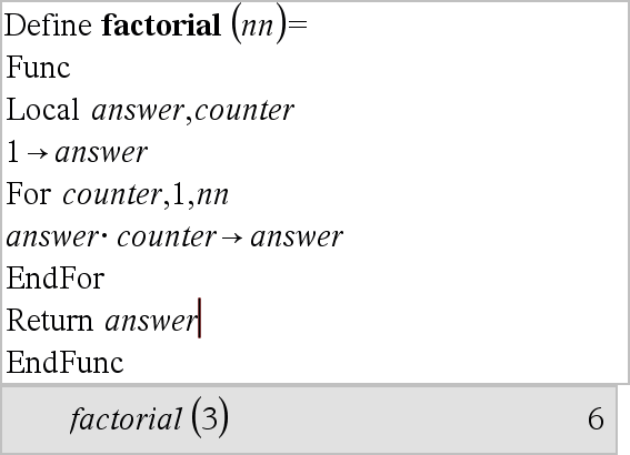
Return [Expr] Returns Expr as the result of the function. Use within a Func...EndFunc block. Note: Use Return without an argument within a Prgm...EndPrgm block to exit a program. Note for entering the example: For instructions on entering multi-line program and function definitions, refer to the Calculator section of your product guidebook. |
|
|
Catalog > |
|
|
right(List1[, Num]) ⇒ list Returns the rightmost Num elements contained in List1. If you omit Num, returns all of List1. |
|
|
right(sourceString[, Num]) ⇒ string Returns the rightmost Num characters contained in character string sourceString. If you omit Num, returns all of sourceString. |
|
|
right(Comparison) ⇒ expression Returns the right side of an equation or inequality. |
|
Catalog > |
|
|
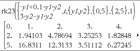
Uses the Runge-Kutta method to solve the system Expr is the right hand side that defines the ordinary differential equation (ODE). SystemOfExpr is a system of right-hand sides that define the system of ODEs (corresponds to order of dependent variables in ListOfDepVars). ListOfExpr is a list of right-hand sides that define the system of ODEs (corresponds to order of dependent variables in ListOfDepVars). Var is the independent variable. ListOfDepVars is a list of dependent variables. {Var0, VarMax} is a two-element list that tells the function to integrate from Var0 to VarMax. ListOfDepVars0 is a list of initial values for dependent variables. If VarStep evaluates to a nonzero number: sign(VarStep) = sign(VarMax-Var0) and solutions are returned at Var0+i*VarStep for all i=0,1,2,… such that Var0+i*VarStep is in [var0,VarMax] (may not get a solution value at VarMax). if VarStep evaluates to zero, solutions are returned at the "Runge-Kutta" Var values. diftol is the error tolerance (defaults to 0.001). |
Differential equation: y'=0.001*y*(100-y) and y(0)=10 To see the entire result, Same equation with diftol set to 1.E−6 System of equations:
with y1(0)=2 and y2(0)=5
|
|
Catalog > |
|
|
root(Value) ⇒ root
root(Value1, Value2) returns the Value2 root of Value1. Value1 can be a real or complex floating point constant or an integer or complex rational constant. Note: See also Nth root template, here. |
|
|
Catalog > |
|
|
rotate(Integer1[,#ofRotations]) ⇒ integer Rotates the bits in a binary integer. You can enter Integer1 in any number base; it is converted automatically to a signed, 64-bit binary form. If the magnitude of Integer1 is too large for this form, a symmetric modulo operation brings it within the range. For more information, see ►Base2, here. |
In Bin base mode:
To see the entire result, |
|
If #ofRotations is positive, the rotation is to the left. If #ofRotations is negative, the rotation is to the right. The default is −1 (rotate right one bit). For example, in a right rotation: |
In Hex base mode:
|
|
Each bit rotates right. 0b00000000000001111010110000110101 Rightmost bit rotates to leftmost. produces: 0b10000000000000111101011000011010 The result is displayed according to the Base mode. |
Important: To enter a binary or hexadecimal number, always use the 0b or 0h prefix (zero, not the letter O). |
|
rotate(List1[,#ofRotations]) ⇒ list Returns a copy of List1 rotated right or left by #of Rotations elements. Does not alter List1. If #ofRotations is positive, the rotation is to the left. If #of Rotations is negative, the rotation is to the right. The default is −1 (rotate right one element). |
In Dec base mode:
|
|
rotate(String1[,#ofRotations]) ⇒ string Returns a copy of String1 rotated right or left by #ofRotations characters. Does not alter String1. If #ofRotations is positive, the rotation is to the left. If #ofRotations is negative, the rotation is to the right. The default is −1 (rotate right one character). |
|
|
Catalog > |
|
|
round(Value1[, digits]) ⇒ value Returns the argument rounded to the specified number of digits after the decimal point. digits must be an integer in the range 0–12. If digits is not included, returns the argument rounded to 12 significant digits. Note: Display digits mode may affect how this is displayed. |
|
|
round(List1[, digits]) ⇒ list Returns a list of the elements rounded to the specified number of digits. |
|
|
round(Matrix1[, digits]) ⇒ matrix Returns a matrix of the elements rounded to the specified number of digits. |
|
|
Catalog > |
|
|
rowAdd(Matrix1, rIndex1, rIndex2) ⇒ matrix Returns a copy of Matrix1 with row rIndex2 replaced by the sum of rows rIndex1 and rIndex2. |
|
|
Catalog > |
|
|
rowDim(Matrix) ⇒ expression Returns the number of rows in Matrix. Note: See also colDim(), here. |
|
|
Catalog > |
|
|
rowNorm(Matrix) ⇒ expression Returns the maximum of the sums of the absolute values of the elements in the rows in Matrix. Note: All matrix elements must simplify to numbers. See also colNorm(), here. |
|
|
Catalog > |
|
|
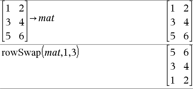
rowSwap(Matrix1, rIndex1, rIndex2) ⇒ matrix Returns Matrix1 with rows rIndex1 and rIndex2 exchanged. |
|
|
Catalog > |
|||||||
|
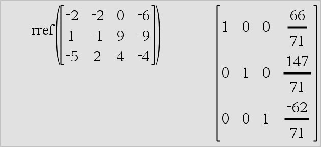
rref(Matrix1[, Tol]) ⇒ matrix Returns the reduced row echelon form of Matrix1. |
|
||||||
|
Optionally, any matrix element is treated as zero if its absolute value is less than Tol. This tolerance is used only if the matrix has floating-point entries and does not contain any symbolic variables that have not been assigned a value. Otherwise, Tol is ignored.
Note: See also ref(), here. |


