In Lesson 22.1 you explored several power series and their relationships to the functions to which they converge. In this lesson you will start with a function and find the power series that converges to that function for values of x near zero. This type of series is called a Maclaurin series.

Finding a Quadratic Polynomial that Approximates a Function Near x = 0

It turns out that finding a second-degree polynomial p(x) = ax² + bx + c that satisfies p(0) = f(0),
p'(0) = f'(0), and p"(0) = f"(0), gives a good approximation to f near x = 0.

The procedure below illustrates the method by finding a quadratic polynomial that satisfies these conditions for the function f(x) = e^x.

• Perform NewProb
• Define f(x)=e^x
• Define p(x)=a*x^2+b*x+c

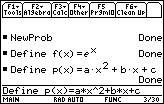
Find the value of c when the two function values are equal at x = 0.

• solve(f(x) = p(x), c) | x=0

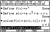
If c = 1, the function and the polynomial have the same value at x = 0, so p(x) = ax² + bx + 1

Set the first derivatives equal and solve for b when x = 0.

• solve(d(f(x), x) = d(p(x), x), b) | x=0

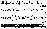
If b = 1, the function and the polynomial will have the same slope at x = 0, so p(x) = ax² + x + 1.

Set the second derivatives equal and solve for a when x = 0.

• solve(d(f(x), x, 2) = d(p(x), x, 2), a) | x=0

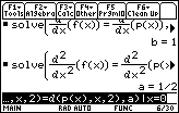
If a = 1/2, the function and the polynomial will have the same concavity at x = 0. Therefore,
p(x) = (1/2)x² + x + 1 approximates y = e^x near x = 0.

Displaying Graphs of the Function and the Approximating Quadratic Polynomial

• Graph the functions y1 = e^x and in a [-10, 10] x [-10, 10] window and set the graphing style of y1 = e^x to "thick"

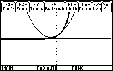
The parabola has the same value, the same slope and the same concavity as y = e^x at x = 0. The quadratic polynomial is a good approximation for y = e^x at x = 0.

22.2.1 Create a table of values for y = e^x and with tblStart = -1 and tbl = 0.1. Compare the values of y = e^x and the quadratic polynomial when x = -0.5 and when x = 0.5.

Click here for the answer.

Outlining the General Procedure of Finding Maclaurin Series

The general idea for finding the coefficients of a power series

that approximates a function

y = f(x)

near x = 0 is first to set the value of the power series equal to the value of f(x) at x = 0 and solve for c₀. Then, set all of the derivatives of the power series (beginning with the first) equal to the corresponding derivative of f(x) at x = 0 and solve for the remaining coefficients of the power series.

The series found is this fashion is called the Maclaurin series for f(x).

Letting f ^(k)(x) represent the kth derivative of f, the coefficient of the term that contains the kth power of x in a Maclaurin series is

This method produces the following power series for y = e^x :

The Maclaurin series above is more than an approximation of e^x, it is equal to e^x on the interval of convergence (– , ).

Every Maclaurin series is centered at 0 and the interval of convergence is centered at 0. When the Maclaurin series approximates a function, the series values and the function values are very close near x = 0.

The partial sum

is the nth-order Maclaurin polynomial for f.

Generating Maclaurin Polynomials on a TI-89

The TI-89 can generate Maclaurin polynomials for a function f using the taylor( command.

Taylor Command The taylor( command, which is the 9th item in the Calc menu of the Home screen, has the following syntax: taylor(expression, var, order) expression represents the function, var represents the variable, and order represents the order of the desired Maclaurin polynomial.

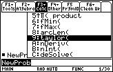
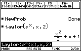
Generate the second-order Maclaurin polynomial for e^x using the taylor( command.

• Perform NewProb
• Open the Calc menu by pressing
• Highlight 9:taylor( by scrolling to the 9th element in the menu

• Paste taylor( to the Edit Line by pressing
• Execute the command taylor(e^x, x, 2)

22.2.2 Use the taylor command to find the fifth-order Maclaurin polynomial for
y = ln(1 + x) and interpret the result. Click here for the answer.

22.2.3 Graph y = ln(1 + x) and the fifth-order polynomial from 22.2.2 together. Click here for the answer.