In this lesson you will model the motion of a particle that moves along the x-axis using parametric equations. The motion of the particle will be illustrated using the animation feature of the TI-83. By developing different parametric equations to model the same movement, you will see that parametric equations that model a particle's movement are not unique.

Suppose a particle moves along the x-axis so that its position is given by the equation below, where t represents time in seconds.

Parametric Equations

You can use your TI-83 to illustrate the motion of the particle by defining its movement with parametric equations, which were explored in Module 4. Displaying the parametric equations in animated graph mode will help determine when the particle is at rest, when it is moving right, and when it is moving left.

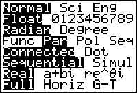
To graph parametric equations on the TI-83 you need to change the graphing mode.

• Display the Mode settings by pressing .
• Select PARAMETRIC graphing mode by highlighting "Par" and pressing .

• Open the Y= editor by pressing .
• Clear any existing equations in the editor.

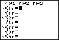
The particle's horizontal position along the x-axis is given by x(t) = 2t³ - 9t² + 12t + 1 and its vertical position is constantly zero because the particle is moving along the x-axis.

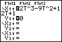
• Set X_1T = 2T^3 - 9T^2 + 12T + 1.
  Notice that pressing enters "T," not "X," when in PARAMETRIC graph mode.
• Set Y_1T = 0.

Independent Y= Editors The Y= editor maintains an independent list of function definitions for each Graph mode. When you return to FUNCTION graphing mode, your y(x) functions are still defined, and upon return to PARAMETRIC graphing mode, the x(t) and y(t) parametric equations will still be stored.

Setting the Graph Style to Animate

When an equation is graphed in Animate style, a small circular icon moves along the path defined by the equation. You can view an animation of the particle's motion by changing the Graph style of the parametric equations.

• Move the cursor left of X_1T by using the left arrow key.
• Change the Graph style to Animated by pressing until you see " ".

Setting the Viewing Window

• Enter the window values [0, 4, 0.1] x [-2, 15, 1] x [-1, 4, 1].

With the values shown, t will initially be 0 and then increase by steps of one tenth until it is 4. For each value of t the position of the particle, as determined by the corresponding x and y-values, will be plotted.

• Display the graph by pressing .

You should see a circular icon move along the x-axis. This circle illustrates the path of the particle over the time interval from t = 0 to t = 4 as defined by x(t) = 2t³ - 9t² + 12t + 1.

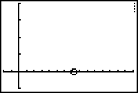
The screen above shows an intermediate view of the animation when the graph is displayed.

You can see the animation again by pressing [DRAW] and selecting 1:ClrDraw.

Slowing the Motion You can slow the motion of the animation by making the value of Tstep smaller in the WINDOW settings.

Animation Using the Trace Feature

The Trace feature can produce a similar animated effect but the speed of the animation is under your control.

• Activate the Trace cursor by pressing .
• Move the Trace cursor along the path of the particle by using the right arrow key.

Try pressing the left or right arrow and holding it down.

Tracing Time

Notice that the right arrow key moves the particle forward in time, which may not always coincide with motion to the right, and the left arrow key moves the cursor back in time, which may not always coincide with motion to the left. The value of t and the x- and y-coordinates are shown at the bottom of the screen as you trace the particle's motion.

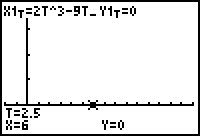
15.1.1 Use the cursor movement keys to estimate the time interval(s) when the particle is moving right. Click here for the answer.

15.1.2 Estimate when the particle is moving left. Click here for the answer.

15.1.3 When does the particle appear to change direction? Click here for the answer.

Illustrating the Path Over Time

The animation on the x-axis is a realistic model for the motion of the particle. However, it's often helpful to have a static graph that can be used to help visualize and study motion. Make the following additions in the Y= editor to better illustrate the motion of the particle over the four-second interval.

Set X_2T = X_1T by following the procedure below.

• Open the Y= editor and move the cursor to the line where X_2T is defined.
• Open the Y-VARS menu by pressing .
• Select "2:Parametric"

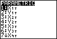
• Paste "X_1T" to the Y= editor where the cursor is positioned.
• Set Y_2T = T.

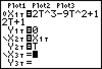
Setting the Path Style

• Move the cursor left of X_2T by using the left arrow key.
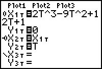
• Press until you see " ," which is the icon for "Path" graphing style. The Path style shows the animation and leaves a trail where the particle has been.

Simultaneous Graphing

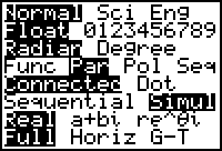
The graphs defined in X_1T, Y_1T and in X_2T, Y_2T can be drawn at the same time by setting the Graph mode to Simultaneous.

• Open the Mode screen with .
• Highlight "Simul" with the cursor movement keys and press .

Displaying the Graphs

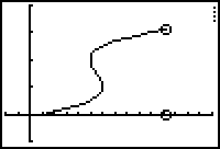
• Display the simultaneously drawn graphs by pressing .
• Pause before the two graphs go off the screen by pressing . Notice the busy indicator (four vertical dots) in the upper right-hand corner of the screen.

• You can continue to display the current graphs by pressing , or you can clear the drawing and restart the animation at t = 0 by pressing [DRAW] .

Notice the advantage that this visualization has over the original "Path" style. Any trail left on a 1-dimensional motion hides changes in direction and doesn't give any information about when the particle is in what position.

15.1.4 Identify the features of the graph that indicate when the particle appears to change direction, and then approximate the times when the particle changes direction. Click here for the answer.

A Different Model of the Particle's Motion

Different parametric equations can be used to make another model of the same particle motion. The functions below represent the same motion shown earlier, but time is now shown on the horizontal axis and the particle's position is represented vertically.

• Clear all the equations defined in the Y= editor.
• Set X_1T = T.
• Set Y_1T = 2T^3 - 9T^2 + 12T + 1.
• Display the graph in a [0, 6, 0.1] x [0, 6, 1] x [-5, 20, 5] window.

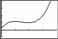
In the graph above, the y-values represent the particle's position and the x-values represent the corresponding times. This model has the advantage of having time as the x-variable and position as the y-variable, which is comparable to the representation normally used in the FUNCTION Graph mode.

Instantaneous Velocity of the Particle

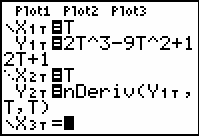
The particle's instantaneous velocity function can be displayed along with its position function. Defining new parametric equations where the x-values represent time and the y-values represent the particle's instantaneous velocity (the derivative of the function in Y_1T) can do this.

• Set X_2T = T.
• Set the graphing style to Dot.
• Set Y_2T = nDeriv(Y_1T,T,T). Recall that nDeriv is in the MATH menu. You could also simply type in the actual derivative for Y_2T, namely, 6T^2-18T+12.

• Graph the equations.

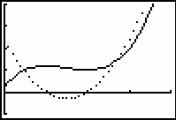
15.1.5 Describe how these graphs show when the particle is moving left, moving right, and at rest. Click here for the answer.