In this lesson you will use graphical and numerical methods to support algebraic conclusions about limits.
The limit of a function may be estimated from a graph of the function or numerically from a table of function values.
The Graphical Approach
Estimate
![]() graphically by using the Trace feature, as described below.
graphically by using the Trace feature, as described below.
- Make sure "Radian" mode is selected in the Mode menu.
- Enter Y1 = sin(X)/X.
-
Select a Zoom Decimal window by pressing
 and selecting 4:ZDecimal.
-
Display function values by pressing
 .
.
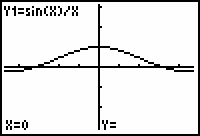
The fact that there is no value beside the y-coordinate shows that Y1 is undefined at x = 0. However, the limit as x approaches 0 of the function is defined because you can get as close to 1 as you want by letting x be close enough to 0.
The limit can be illustrated by using the Trace feature.
-
Move the Trace cursor just to the right of x = 0 by pressing

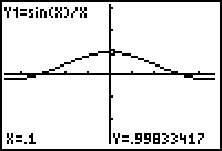
- Continue to use Trace, or the Value feature in the CALCULATE menu to find the function values at x = 0.01, x = -0.1, and x = -0.01.
The graph and displayed values provide evidence that when x is close to 0,
![]() is close to 1, or
is close to 1, or
Numerical Approach
The Table feature of the TI-83 can be used to evaluate
![]() for values of x close to 0.
for values of x close to 0.
-
Enter the Table Setup menu by pressing
 [TBLSET]. [TBLSET] is above
 .
.
-
Select "Ask" mode for the independent variable by moving to the line that begins with "Indpnt", highlighting "Ask" and pressing
 .
.
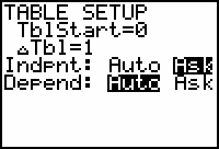
In the ASK mode you can enter any value you choose for x in the table and the calculator will generate the corresponding y value for functions selected in the Y= editor.
-
Press
 [TABLE] and enter the values of 0.1, 0.01, 0.001, -0.001, -0.01, and -0.1 for x. Press
 after each x value to see the corresponding y value.
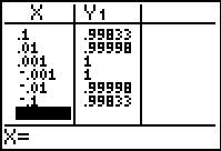
The table provides numerical evidence that
![]() .
.
|
|||
|
|
|||
|
|||
|
|
|||
The Sandwich Theorem
The Sandwich theorem is used in many calculus books to prove that
![]() . Consider the following argument:
. Consider the following argument:
-
It can be shown by a geometrical argument that
 for
for

-
Because the left and right terms in the inequality above approach 1 as
 , it must follow that the middle term must also approach 1.
This argument is called the Sandwich Theorem because the values of sin(x)/x are "sandwiched" between the values of cos(x) and 1.
Simultaneous Graphing
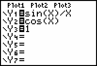
The Sandwich theorem can be illustrated by graphing the three terms of the compound inequality simultaneously.
- Enter the three functions shown in the Y= editor, as shown below.
-
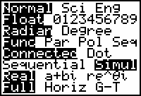
Change the graph format to simultaneous by pressing
 , highlighting "Simul" and pressing
 .
.
- Display the graphs of the functions in a [-3, 3, 1] x [-1, 2, 1] window.
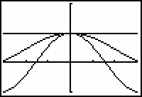
The simultaneous convergence of three graphs to 1 around x = 0 illustrates the Sandwich theorem's argument that
![]() .
.
Redrawing the Graphs
You can see the three functions converge again using the Clear Draw command.
-
Redraw the graphs by pressing
 [DRAW]
 .
.
[DRAW] is above in the third row's third column of keys.
Left- and Right-Hand Limits
The notation
![]() represents a right-hand limit and it is read "the limit of
represents a right-hand limit and it is read "the limit of
![]() as x approaches 0 from the right." It represents the value approached by
as x approaches 0 from the right." It represents the value approached by
![]() as x approaches 0 through positive values, which are to the right of 0, as shown below.
as x approaches 0 through positive values, which are to the right of 0, as shown below.
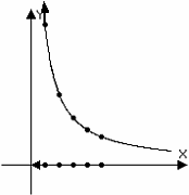
The diagram illustrates the x-values approaching 0 through positive values and the corresponding values of
![]() .
.
The notation
![]() represents a left-hand limit and it is read "the limit of
represents a left-hand limit and it is read "the limit of
![]() as x approaches 0 from the left." It represents the value approached by
as x approaches 0 from the left." It represents the value approached by
![]() as x approaches 0 through negative values, which are to the left of 0, as shown below.
as x approaches 0 through negative values, which are to the left of 0, as shown below.
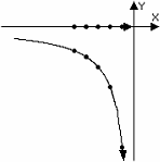
The diagram illustrates the x-values approaching 0 through negative values and the corresponding values of
![]() .
.
Using the Trace Feature
The Trace feature may be used to estimate these limits. As the Trace cursor moves along a curve, the x- and y-values appear at the bottom of the Graph screen.
Look at the y-values of
![]() as x approaches 0 from the left and from the right by using the Trace feature.
as x approaches 0 from the left and from the right by using the Trace feature.
- Graph y = 1/x in a [-3, 3, 1] x [-10, 10, 1] window.
-
Activate the Trace cursor by pressing
 .
.
-
Display coordinates of the graph by repeatedly pressing
 or
or
 to move the cursor along the curve
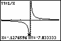
Moving the Trace cursor toward zero from the left and from the right provides graphical and numeric reinforcement for the left- and right-hand limits shown below.
Entering a Specific x-Value
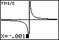
While the Trace cursor is active, you can move it to a particular point by typing in the x-coordinate of the desired point. For example, move to the point with x = -0.001 while the Trace cursor is active.
-
Enter -0.001.
This value should appear by "X=" in the lower left corner of the screen.
-
Execute the Trace command by pressing
 .
.
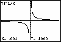
The cursor is not visible because it is below the viewing window, but the coordinates of the cursor are shown giving further evidence that
![]() .
.