A function can be described as a black box with an input and a corresponding output. Each input value x enters the box and then undergoes a transformation that produces a corresponding output value y. For continuous functions the output values will be close to a particular value of y if the input values are "close enough" to the corresponding value of x. In this lesson you will quantify the concept of closeness for a specific function.

Investigating Tolerances of

For , y is close to 2 when x is close to 3.

An example of the type of question that is key to understanding limits is

How close should x be to 3 to ensure that y is within 0.1 of 2?

Graphing the Function and Output Bounds

Begin the investigation by graphing the function and the two horizontal lines that represent the y-tolerances: one line that is 0.1 below y = 2 and the other line that is 0.1 above y = 2.

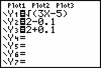
• Enter the functions below in the Y= editor.



Y₂ = 2 - 0.1, the horizontal line 0.1 units below y = 2

Y₃ = 2 + 0.1, the horizontal line 0.1 units above y = 2

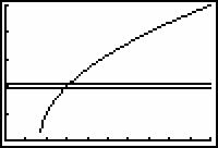
Display the graph of the function to see its basic shape and the graphs of the two horizontal lines that represent the output tolerance. Use a [0, 10, 1] x [0, 5, 1] viewing window.

A Better View

The region of the graph where y is 0.1 unit away from 2 can be better seen using a viewing window with values close to x = 3 and y = 2.

• Redraw the graph in a [2.8, 3.2, 0.1] x [1.8, 2.2, 0.1] viewing window.

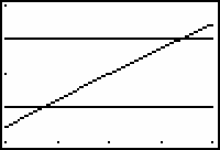
The graph of appears to be a diagonal line rather than a curve because a small portion of the graph has been magnified to fill the window. The points of intersection of the function and the two horizontal lines that are 0.1 away from 2 determine the endpoints of the x-interval where the values of the function are within 0.1 of 2.

Finding the x-Tolerances Using the Intersection Feature

The x-coordinates of the points where the graph of the function intersects the horizontal lines determine how close x needs to be to 3 so that y is within 0.1 of 2. The Intersect feature in the CALCULATE menu of the Graph screen can be used to find the intersection points.

• Display the CALCULATE menu by pressing [CALC]. [CALC] is above .

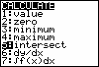
• Select 5:intersect.

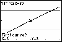
To find the x-coordinate of the point of intersection of Y₂ = 1.9 (the lower bound of the y-tolerance) and (the graph of the function), you need to specify the two curves.

Selecting the Two Intersecting Curves

The cursor is on the function Y₁, as indicated by the "Y1" in the upper left portion of the screen and the blinking cursor on the graph.

• Select this function as one of the curves by pressing .

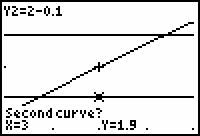
The small + shown on the graph of Y₁ indicates that it is the first curve selected. The cursor is on the lower horizontal line to indicate that that line is currently chosen and it is blinking to indicate that it has not been selected. Note that "Y2" is shown in the upper left portion of the screen indicating that the current position of the cursor is on the graph of Y₂.

• Designate the lower line (Y₂) as the second curve by pressing .

Specifying an Initial Guess

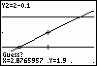
The TI-83 will prompt you for an initial guess of the point of intersection.

• Move the cursor close to the point of intersection with the left arrow key, .

• Specify the initial guess by pressing .

The calculator improves upon your initial guess and displays a good approximation of the point of intersection.

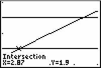
The x-coordinate of the point of intersection is approximately 2.87.

Finding the Second Point of Intersection

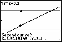
Now find the point where the graph of the function intersects the upper horizontal line, Y₃ = 2.1.

• Select the Intersect feature from the CALCULATE menu by pressing [CALC] .
• Select the function as the first curve by pressing .
• Move the cursor to the top line by pressing .

• Select Y₃ as the second curve by pressing .
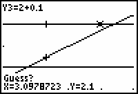
• Move the cursor close to the intersection point by pressing repeatedly.

• Select an initial guess for the point by pressing .

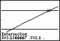
The x-coordinate of this intersection point is approximately 3.1366667.

You can conclude that if x is between 2.87 and 3.1366667, y will be within 0.1 of 2. But that was not the original question.

The original question was

How close should x be to 3 to ensure that y is within 0.1 of 2?

It looks like there are two different answers. The left value of 2.87 is 0.13 from 3. The right value of 3.1366667 is 0.1366667 from 3.

6.1.1 Which tolerance for x, 0.13 or 0.1366667, will ensure that y is within 0.1 of 2 when x is close to 3? Click here for the answer.

Smaller y Tolerances

6.1.2 For , how close should x be to 3 so that y is within 0.01 of 2? Click here for the answer.