Statistics

% t     v

% t displays a menu with the following options:

•

1-Var Stats analyzes data from 1 data set with 1 measured variable, x.

•

2-Var Stats analyzes paired data from 2 data sets with 2 measured variables—x, the independent variable, and y, the dependent variable.

•

StatVars displays a secondary menu of statistical variables. The StatVars menu only appears after you have calculated 1-Var or 2-Var stats. Use $ and # to locate the desired variable, and press < to select it.

Variables	Definition
n	Number of x or (x,y) data points.
Ï or Ð	Mean of all x or y values.
Sx or Sy	Sample standard deviation of x or y.
Îx or Îy	Population standard deviation of x or y.
x or y	Sum of all x or y values.
x2 or y2	Sum of all x2 or y2 values.
xy	Sum of (x…y) for all xy pairs.
a	Linear regression slope.
b	Linear regression y-intercept.
r	Correlation coefficient.
x' (2-Var)	Uses a and b to calculate predicted x value when you input a y value.
y' (2-Var)	Uses a and b to calculate predicted y value when you input an x value.

To define statistical data points:

1.

Enter data in L1, L2, or L3. (See Data Editor and List Conversions.)

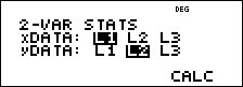
2.

Press % t. Select 1-Var or 2-Var and press <.

3.

Select L1, L2, or L3, and the frequency.

4.

Press < to display the menu of variables.

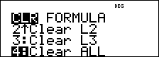
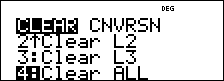
5.

To clear data, press v v, select a list to clear, and press <.

Examples

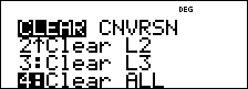
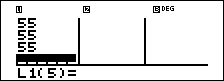
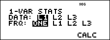
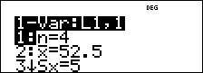
1-Var: Find the mean of {45,55,55,55}

Clear all data	v v $ $ $
Data	< 45 $ 55 $ 55 $ 55 <
Stat	% t
	1 $ $
	<
Stat Var	% s % t 3
	2 <
	V 2 <

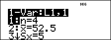
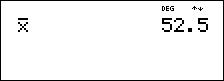
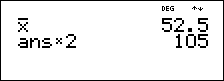
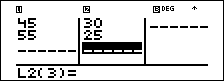
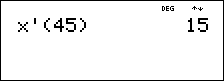
2-Var: Data: (45,30), (55,25); Find: x '(45)

Clear all data	v v $ $ $
Data	< 45 $ 55 $ " 30 $ 25 $
Stat	% t (Your screen may not show 3:StatVars if you did not previously perform a calculation.)
	2 $ $
	<
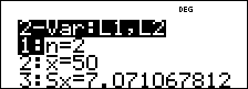
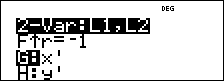
	% s % t 3 # #
	< 45 E <

³ Problem

For her last four exams, Ada earned the following scores.

Test No.	1	2	3	4
Score	73	94	85	78

1.

Find Ada’s average grade on the four exams.

2.

Ada found an error in the two of her test scores. Test 2 was changed to 88 and Test 4 was changed to 84. Find Ada's new average grade of the four exams.

3.

What do you notice about Ada's average grades before the point change and after the point change?

Clear all data	v v 4
Data	73 $ 94 $ 85 $ 78 $
	% t
	1 $ $ < The average grade is 82.5.
	v $ 88 $ $ 84 $
	% t 1
	$ $ < The new average grade is 82.5.

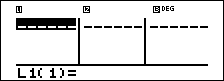
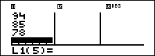
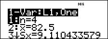
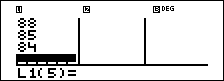
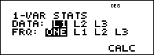
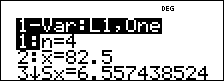
Ada's average did not change. It remained 82.5 after the grade corrections.

The reason the average did not change is that Test 2 had a decrease of 6 points while Test 4 had an increase of 6 points. Overall, the total points for all four tests remained the same (330 points).

³ Problem

The table below gives the results of a braking test.

Test No.	1	2	3	4
Speed (kph)	33	49	65	79
Distance (m)	5.30	14.45	20.21	38.45

Using the relationship between these data points, estimate the stopping distance required for a vehicle traveling at 55 kph.

A hand-drawn scatter plot of these data points suggest a linear relationship. The TI-34 MultiView™ calculator uses the least squares method to find the line of best fit, y'=ax'+b, for data entered in lists.

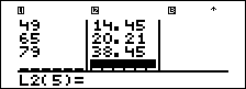
v v 4
33 $ 49 $ 65 $ 79 $ " 5.3 $ 14.45 $ 20.21 $ 38.45 $
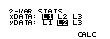
% t
2 $ $
<
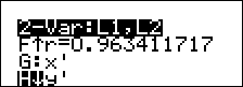
Press $ to view a and b.

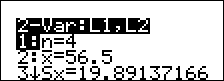
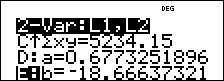
This line of best fit, y ' = 0.6773251896x '-18.66637321 models the linear trend of the data.

% s % t 3 #
< 55 E <

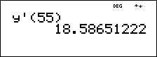
The linear model gives an estimated braking distance of 18.59 meters for a vehicle traveling at 55 kph.