Teacher Information
How might your classes change with a CBR™ 2 motion sensor?
The CBR™ 2 motion sensor is an easy-to-use system with features that help you integrate it into your lesson plans quickly and easily.
The CBR™ 2 motion sensor offers significant improvements over other data-collection methods you may have used in the past. This, in turn, may lead to a restructuring of how you use class time, as your students become more enthusiastic about using real-world data.
|
•
|
You’ll find that your students feel a greater sense of ownership of the data because they actually participate in the data-collection process rather than using data from textbooks, periodicals, or statistical abstracts. This impresses upon them that the concepts you explore in class are connected to the real world and aren’t just abstract ideas. But it also means that each student will want to take his or her turn at collecting the data. |
|
•
|
Data collection with CBR™ 2 motion sensor is considerably more effective than creating scenarios and manually taking measurements with a ruler and stopwatch. Since more sampling points give greater resolution and since a motion sensor is highly accurate, the shape of curves is more readily apparent. You will need less time for data collection and have more time for analysis and exploration. |
|
•
|
With CBR™ 2 motion sensor students can explore the repeatability of observations and variations in what-if scenarios. Such questions as “Is it the same parabola if we drop the ball from a greater height?” and “Is the parabola the same for the first bounce as the last bounce?” become natural and valuable extensions. |
|
•
|
The power of visualization lets students quickly associate the plotted list data with the physical properties and mathematical functions the data describes. |
Other changes occur once the data from real-world events is collected. CBR™ 2 motion sensor lets your students explore underlying relationships both numerically and graphically.
Explore data graphically
Use automatically generated plots of distance, velocity, and acceleration with respect to time for explorations such as:
|
•
|
What is the physical significance of the y-intercept? the x-intercept? the slope? the maximum? the minimum? the derivatives? the integrals? |
|
•
|
How do we recognize the function (linear, parabolic, etc.) represented by the plot? |
|
•
|
How would we model the data with a representative function? What is the significance of the various coefficients in the function (e.g., AX2 + BX + C)? |
Explore data numerically
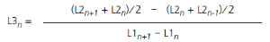
Your students can employ statistical methods (mean, median, mode, standard deviation, etc.) appropriate for their level to explore the numeric data. When you exit the Vernier EasyData® App, a prompt reminds you of the lists in which time (L1), distance (L2), velocity L3), and acceleration (L4) are stored.
CBR™ 2 motion sensor plots—connecting the physical world and mathematics
The plots created from the data collected by Vernier EasyData® App are a visual representation of the relationships between the physical and mathematical descriptions of motion. Students should be encouraged to recognize, analyze, and discuss the shape of the plot in both physical and mathematical terms. Additional dialog and discoveries are possible when functions are entered in the Y= editor and displayed with the data plots.
Performing the same calculations as CBR™ 2 motion sensor is an interesting classroom activity.
|
1.
|
Collect sample data. Exit the Vernier EasyData® App. |
|
2.
|
Use the sample times in L1 in conjunction with the distance data in L2 to calculate the velocity of the object at each sample time. Then compare the results to the velocity data in L3. |
|
3.
|
Use the velocity data in L3 (or the student-calculated values) in conjunction with the sample times in L1 to calculate the acceleration of the object at each sample time. Then compare the results to the acceleration data in L4. |
|
•
|
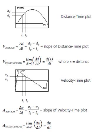
A Distance-Time plot represents the approximate position of an object (distance from the CBR™ 2 motion sensor) at each instant in time when a sample is collected. y-axis units are meters or feet; x-axis units are seconds. |
|
•
|
A Velocity-Time plot represents the approximate speed of an object (relative to, and in the direction of, the CBR™ 2 motion sensor) at each sample time. y-axis units are meters/àsecond or feet/àsecond; x-axis units are seconds. |
|
•
|
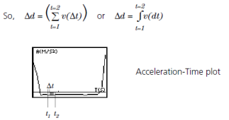
An Acceleration-Time plot represents the approximate rate of change in speed of an object (relative to, and in the direction of, the CBR™ 2 motion sensor) at each sample time. y-axis units are metersàsecond2 or feetàsecond2; x-axis units are seconds. |
|
•
|
The first derivative (instantaneous slope) at any point on the Distance-Time plot is the speed at that instant. |
|
•
|
The first derivative (instantaneous slope) at any point on the Velocity-Time plot is the acceleration at that instant. This is also the second derivative at any point on the Distance-Time plot. |
|
•
|
A definite integral (area between the plot and the x-axis between any two points) on the Velocity-Time plot equals the displacement (net distance traveled) by the object during that time interval. |
|
•
|
Speed and velocity are often used interchangeably. They are different, though related, properties. Speed is a scalar quantity; it has magnitude but no specified direction, as in “6 feet per second.” Velocity is a vector quantity; it has a specified direction as well as magnitude, as in “6 feet per second due North.” |
A typical CBR™ 2 motion sensor Velocity-Time plot actually represents speed, not velocity. Only the magnitude (which can be positive, negative, or zero) is given. Direction is only implied. A positive velocity value indicates movement away from the CBR™ 2 motion sensor; a negative value indicates movement toward the CBR™ 2 motion sensor.
The CBR™ 2 motion sensor measures distance only along a line from the sensor. Thus, if an object is moving at an angle to the line, it only computes the component of velocity parallel to this line. For example, an object moving perpendicular to the line from the CBR™ 2 motion sensor shows zero velocity.
The mathematics of distance, velocity, and acceleration
The area under the Velocity-Time plot from t1 to t2 = @d = (d2Md1) = displacement from t1 to t2 (net distance traveled).
Web-site resources
At TI’s Web Site, education.ti.com, you will find:
|
•
|
a listing of supplemental material for use with the CBR™ 2 motion sensor and TI graphing calculators |