Lesson 3.1 and Lesson 3.2 discussed transformations and Lesson 3.3 explored finding the solutions of transformed exponential functions. This lesson will investigate finding the equation that models a set of data.

The Cooling Problem

A cup of hot water was left on a kitchen table to cool. The initial temperature of the water was 77.8°C and the room temperature in the kitchen was 23°C. The following table shows data for the water as it cooled.

Enter the data into lists.

• Clear any functions in the Y= editor.
• Enter the data in L₁ and L₂ in the List editor.

The lists are accessed by pressing and selecting 1:Edit.

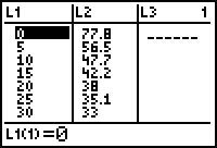
Display the scatter plot of the data.

• Go to the STAT PLOT Setup menu and select Plot1.
• Turn Plot1 On and select the scatter plot icon for the Type.
• Select L₁ for the Xlist and L₂ for the Ylist.
• Select the little box "" for the Mark in STAT PLOT Setup.
• Display the scatter plot of the data in a [-10, 100, 10] x [-10, 90, 10] window.

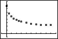
The scatter plot looks like an exponential decay graph with one important difference: the horizontal asymptote for the scatter plot appears to be about y = 23 while the horizontal asymptote for an exponential decay curve is y = 0.

If the scatter plot is shifted down 23, the resulting scatter plot appears to approximate an exponential decay curve. You may calculate an exponential regression equation for the transformed scatter plot and then shift the equation up 23 units to fit the original scatter plot.

Shifting the Scatter Plot Down

Shift the scatter plot down 23 units by subtracting 23 from each L₂-value.

• Open the List editor by pressing .
• Clear L₃ if needed
• Place the cursor on the heading of L₃ by pressing the up arrow key until the list name is highlighted.
• Enter L₂ - 23 into the heading of L₃
  [L₂] is the command above .

Notice as you type that the expression appears in the edit line at the bottom of the screen.

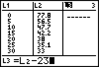
• Execute the command by pressing .

Every element of L₂ is reduced by 23 and the corresponding value stored in L₃.

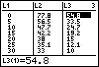
Display the transformed scatter plot with the original scatter plot.

• Return to the STAT PLOT Setup menu and select Plot2.
• Turn Plot 2 On and select the scatter plot icon for the Type.
• Select L₁ for the Xlist and L₃ for the Ylist.

• Display both scatter plots by pressing

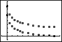
Calculate the exponential regression equation for the transformed scatter plot.

• Return to the Home screen by pressing [QUIT].
• Open the STAT CALC menu by pressing .
• Scroll down to 0:ExpReg using the arrow keys.

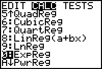
• Paste the ExpReg command to the Home screen by pressing .
• Complete the command ExpReg L₁, L₃, Y₁ by pressing [L₁] [L₃]

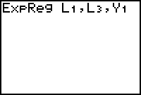
• Execute the command by pressing .

The equation is calculated, displayed on the Home screen and stored in Y₁.

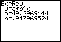
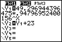
The equation that fits the transformed data is approximately y = 49.3(0.948)^x. Shift this equation up 23 to fit the original data by adding 23: y = 49.3(0.948)^x + 23.

• Enter Y₂ = Y₁ + 23 in the Y= editor. Notice that this uses all the decimal places stored in the calculator for the regression equation instead of the approximation.

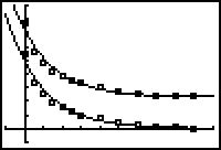
Press to display both equations along with the scatter plots.

3.4.1 Estimate the time needed for the water to cool to 30°C using the table of values of the transformed regression equation. Click here for the answer.