You can study linear and non-linear differential equations and systems of ordinary differential equations (ODEs), including logistic models and Lotka-Volterra equations (predator-prey models). You can also plot slope and direction fields with interactive implementations of Euler and Runge-Kutta methods.
|
|
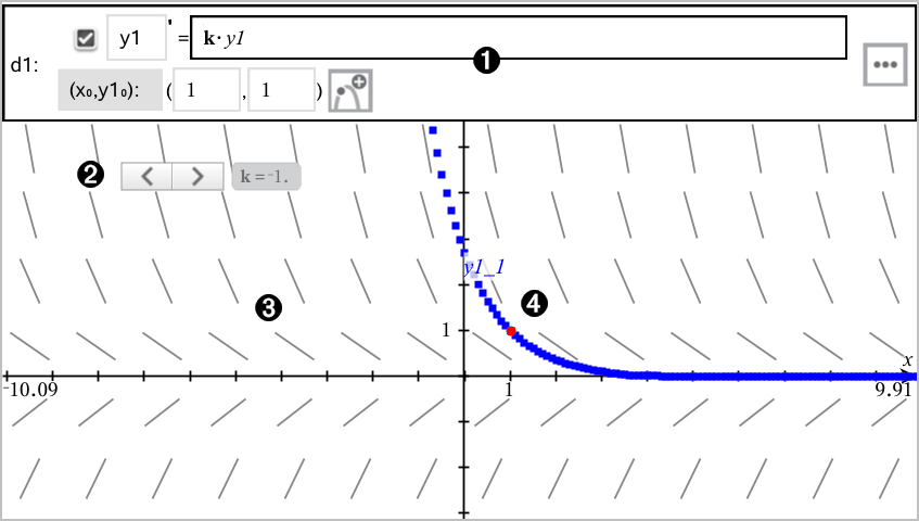
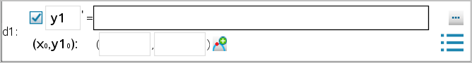
ODE entry line:
|
||||||||||||
|
|
Slider to vary coefficient k of the ODE |
||||||||||||
|
|
Slope field |
||||||||||||
|
|
A solution curve passing through the initial condition |
| 1. | From the Graph Entry/Edit menu, select Diff Eq. |
The ODE is automatically assigned an identifier, such as “y1.”
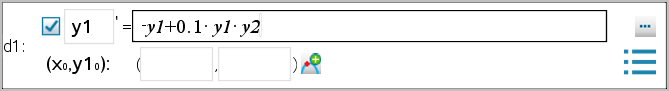
| 2. | Move to the relation field and enter the expression that defines the relation. For example, you might enter -y1+0.1*y1*y2. |
| 3. | Enter the initial condition for the independent value x0 and for y10. |
Note: The x0 value(s) are common to all the ODEs in a problem but can be entered or modified only in the first ODE.
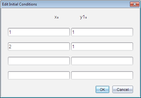
| 4. | (Optional) To study multiple initial conditions for the current ODE, click Add Initial Conditions  and enter the conditions. and enter the conditions. |
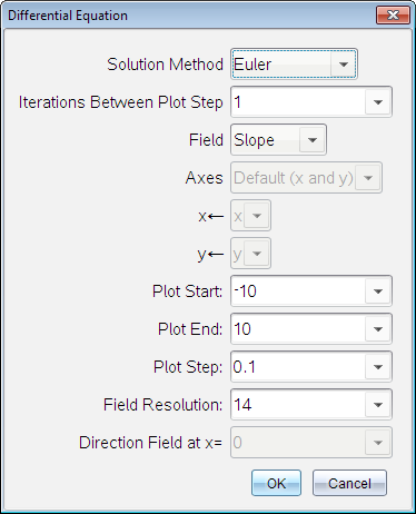
| 5. | Tap Edit Parameters  to set the plot parameters. Select a numerical Solution Method, and then set any additional parameters. You can change these parameters anytime. to set the plot parameters. Select a numerical Solution Method, and then set any additional parameters. You can change these parameters anytime. |
| 6. | Click OK. |
| 7. | To enter additional ODEs, press the down arrow to display the next ODE edit field. |
As you move among defined ODEs, the graph is updated to reflect any changes. One solution to the ODE is graphed for each IC specified for each shown ODE (selected by check box).
|
Solution Method |
Selects Euler or Runge-Kutta as the numerical solution method. |
|||||||||
|
Iterations Between Plot Step |
Computational accuracy for Euler solution method only. Must be an integer value >0. To restore the default, select the down-arrow and select Default. |
|||||||||
|
Error Tolerance |
Computational accuracy for Runge-Kutta solution method only. Must be a floating-point value |1×10-14. To restore the default, select the down-arrow and select Default. |
|||||||||
|
Field |
None - No field is plotted. Available for any number of ODEs, but required if three or more 1st-order ODEs are active. Graphs a combination of the solution and/or values of one or more ODEs (according to user-configured Axes settings). Slope - Plots a field representing the family of solutions to a single 1st-order ODE. Exactly one ODE must be active. Sets Axes to Default (x and y). Sets Horizontal axis to x (the independent variable). Sets Vertical axis to y (the solution to the ODE). Direction - Graphs a field in the phase plane representing the relationship between a solution and/or values of a system of two 1st‑order ODEs (as specified by the CustomAxes setting). Exactly two ODEs must be active. |
|||||||||
|
Axes |
Default (x and y) - Plots x on the x axis and y (the solutions to the active differential equations) on the y axis. Custom - Lets you select the values to be plotted on the x and y axes respectively. Valid entries include:
|
|||||||||
|
Plot Start |
Sets the independent variable value at which the solution plot starts. |
|||||||||
|
Plot End |
Sets the independent variable value at which the solution plot stops. |
|||||||||
|
Plot Step |
Sets the increment of the independent variable at which values are plotted. |
|||||||||
|
Field Resolution |
Sets the number of columns of field rendering elements (line segments) used to draw a slope or direction field. You can change this parameter only if Field = Direction or Slope. |
|||||||||
|
Direction Field at x= |
Sets the independent variable value at which a direction field is drawn when plotting non-autonomous equations (those that refer to x). Ignored when plotting autonomous equations. You can change this parameter only if Field = Direction. |


