Utilisez les exemples de scripts suivants pour vous familiariser avec les méthodes décrites à la section Référence. Par ailleurs, ces exemples comprennent plusieurs scripts TI-Innovator™ Hub et TI-Innovator Rover™ qui faciliteront votre prise en main du langage TI-Python.
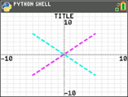
import ti_plotlib as plt
plt.cls()
plt.window(-10,10,-10,10)
plt.axes("on")
plt.grid(1,1,"dot")
plt.title("TITLE")
plt.pen("medium","solid")
plt.color(28,242,221)
plt.pen("medium","dash")
plt.line(-5,5,5,-5,"")
plt.color(224,54,243)
plt.line(-5,-5,5,5,"")
plt.show_plot()
Appuyez sur ‘ pour afficher l'invite du Shell.
Tout d'abord, saisissez deux listes dans le système d'exploitation (OS) CE. Puis, par exemple, calculez [stat] CALC 4:LinReg(ax+b) pour vos listes. Cela permet de stocker l'équation de régression dans RegEQ dans l'OS. Voici un script destiné à rappeler RegEQ dans l'expérience Python.
# Exemple d'utilisation de recall_RegEQ()
from ti_system import *
reg=recall_RegEQ()
print(reg)
x=float(input("Input x = "))
print("RegEQ(x) = ",eval(reg))
import ti_plotlib as plt
# intensité du courant
I = [0.0, 0.9, 2.1, 3.1, 3.9, 5.0, 6.0, 7.1, 8.0, 9.2, 9.9, 11.0,11.9]
# Convertir des milliampères en ampères
for n in range (len(I)):
I[n] /= 1000
# tension
U = [0, 1, 2, 3.2, 4, 4.9, 5.8, 7, 8.1, 9.1, 10, 11.2, 12]
plt.cls()
plt.auto_window(I,U)
plt.pen("thin","solid")
plt.axes("on")
plt.grid(.002,2,"dot")
plt.title("Loi d'Ohm")
plt.color (0,0,255)
plt.labels("I","U",11,2)
plt.scatter(I,U,"x")
plt.color (255,0,0)
plt.pen("thin","dash")
plt.lin_reg(I,U,"center",2)
plt.show_plot()
plt.cls()
a=plt.a
b=plt.b
print ("a =",round(plt.a,2))
print ("b =",round(plt.b,2))
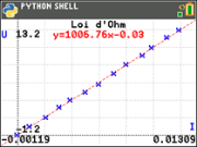
Appuyez sur ‘ pour afficher l'invite du Shell.
import ti_plotlib as plt
#Après avoir exécuté ce script, appuyez sur [annul] pour effacer l'écran
def f(x):
••return 3*x**2-.4
def g(x):
••return -f(x)
def plot(res,xmin,xmax):
••#configurer l'écran graphique
••plt.window(xmin,xmax,xmin/1.5,xmax/1.5)
••plt.cls()
••gscale=5
••plt.grid((plt.xmax-plt.xmin)/gscale*(3/4),(plt.ymax-plt.ymin)/gscale,"dash")
••plt.pen("thin","solid")
••plt.color(0,0,0)
••plt.axes("on")
••plt.labels("abscisse"," ordonnee",6,1)
••plt.pen("medium","solid")
# représenter les fonctions f et g
dX=(plt.xmax -plt.xmin)/res
x=plt.xmin
x0=x
••for i in range(res):
••••plt.color(255,0,0)
••••plt.line(x0,f(x0),x,f(x),"")
••••plt.color(0,0,255)
••••plt.plot(x,g(x),"o")
••••x0=x
••••x+=dX
••plt.show_plot()
#plot(résolution,xmin,xmax)
plot(30,-1,1)
# Créer un graphique avec les paramètres (résolution,xmin,xmax)
# Après avoir effacé le premier graphique, appuyez sur la touche [var]. La fonction plot() permet de modifier les paramètres d’affichage (résolution,xmin,xmax).
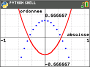
Appuyez sur ‘ pour afficher l'invite du Shell.
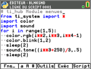
Voir : [Fns…]>Modul: module ti_hub
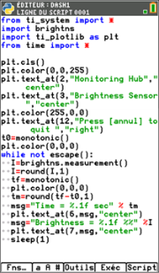
from ti_system import *
import brightns
import ti_plotlib as plt
from time import *
plt.cls()
plt.color(0,0,255)
plt.text_at(2,"Monitoring Hub","center")
plt.text_at(3,"Brightness Sensor","center")
plt.color(255,0,0)
plt.text_at(12,"Press [annul] to quit ","right")
t0=monotonic()
plt.color(0,0,0)
while not escape():
••I=brightns.measurement()
••I=round(I,1)
••tf=monotonic()
••plt.color(0,0,0)
••tm=round(tf-t0,1)
••msg="Time = %.1f sec" % tm
••plt.text_at(6,msg,"center")
••msg="Brightness = %.1f %%" %I
••plt.text_at(7,msg,"center")
••sleep(1)
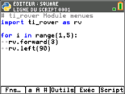
Voir : [Fns…]>Modul module ti_rover
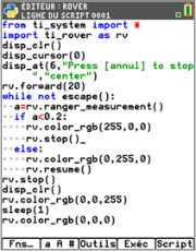
from ti_system import *
import ti_rover as rv
disp_clr()
disp_cursor(0)
disp_at(6,"Press [annul] to stop","center")
rv.forward(20)
while not escape():
••a=rv.ranger_measurement()
••if a<0.2:
••••rv.color_rgb(255,0,0)
••••rv.stop()
••else:
••••rv.color_rgb(0,255,0)
••••rv.resume()
rv.stop()
disp_clr()
rv.color_rgb(0,0,255)
sleep(1)
rv.color_rgb(0,0,0)
Voir : [Fns…]>Modul: module ti_hub
Voir : [Fns…]>Modul module ti_rover
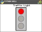
from ti_draw import *
from ti_image import *
from time import *
clear()
# Pixel screen upper left (0,0) to (319,209)
draw_text(100,20,"Traffic Light")
set_pen("medium","solid")
draw_rect(120,25,80,175)
set_color(192,192,192)
fill_rect(120,25,80,175)
set_color(128,128,128)
draw_circle(160,55,22)
draw_circle(160,110,22)
draw_circle(160,165,22)
def off(x,y):
••set_color(169,169,169)
••fill_circle(x,y,22)
••set_color(128,128,128)
••draw_circle(x,y,22)
for i in (1,20,1):
# Green
••set_color(51,165,50)
••fill_circle(160,165,22)
••sleep(3)
••off(160,165)
# Yellow
••set_color(247,239,10)
••fill_circle(160,110,22)
••sleep(2)
••off(160,110)
# Red
••set_color(255,0,0)
••fill_circle(160,55,22)
••sleep(3)
••off(160,55)
••show_draw()