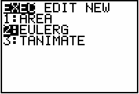
This lesson investigates finding solutions to differential equations by analytical and graphical methods. It also explores finding solutions to initial-value problems. You will use a TI-83 program called EULERG to graph solutions to differential equations.

Definition of a Differential Equation

An equation containing a derivative is called a differential equation. For example, y ' = 2x is a differential equation because it contains the derivative y '. Such equations occur often in real-world applications.

Solutions to Differential Equations

A solution to a differential equation is a function that satisfies the differential equation. There is usually more than one solution to any differential equation. Each of the functions shown below is a solution to the differential equation y ' = 2x because each makes the differential equation true.

y₁ = x²

y₂ = x² + 1

y₃ = x² - 3

These particular solutions, as well as all other solutions to the differential equation y ' = 2x, can be found by using the power rule for integrals.

where C can be any real number. This family of functions is called the general solution to the differential equation.

The solution may be verified by substituting the solution into the original differential equation.
.

Solutions to y ' = f (x)

Solutions to differential equations of the form y ' = f (x) may be found by evaluating but solutions to differential equations of other forms require other techniques.

20.2.1 Solve the differential equation by using the power rule for integrals.

Click here for the answer.

Initial Conditions and Initial-Value Problems

Suppose you need the particular function that satisfies the differential equation y ' = 2x with the condition that y(0) = 1, that is, y = 1 when x = 0. The condition y(0) = 1 is called an initial condition and a differential equation with an initial condition is called an initial-value problem.

The general solution to the differential equation y ' = 2x is y = x² + C.

The value of C can be found by substituting the initial values x = 0 and y = 1.

1 = 0² + C
C = 1

So, the desired particular solution is y = x² + 1.

Any one specific solution of a differential equation is called a particular solution because it is just one solution out of many. In elementary initial value problems, the initial condition selects one particular solution from the family of all solutions.

20.2.2 Solve the initial-value problem, , y(1) = 1.

Click here for the answer.

Graphical Solutions to Differential Equations

You can use a TI-83 program called EULERG to graph approximate solutions to initial-value problems without finding the analytic solution.

Downloading the Program to Your Computer

• Click here to download EULERG to your computer.
• Choose to save the file.
• Save the file on your local hard disk in a folder that you can access later.

Transferring the Program to the TI-83

Click here to get information about how to obtain the needed cable and review the procedure to transfer the program from your computer to your calculator.

• Send the EULERG program from your computer to your TI-83.

Graphing Solutions to Differential Equations

Graph an approximate solution to the initial value problem y' = 2x with the condition that y(0) = 1 by following the procedure outlined below.

The program EULERG requires that you enter the differential equation into Y₁ in the Y= editor and select an appropriate viewing window for the solution before you run the program.

• Enter Y₁ = 2X.
• Enter a [0, 3, 1] x [-1, 10, 1] viewing window.

Running EULERG

• Go to the Home screen and clear it.
• Open the Program menu by pressing .

• Select EULERG. This should paste the command "prgmEULERG" to the Home screen.
• Press to execute the program.
• Enter 0 for INITIAL X.
• Enter 1 for Y(INITIAL X), the y-value for the initial x-value.
• Enter 0.01 for STEP SIZE.

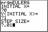
After you enter the STEP SIZE the TI-83 will display a graph.

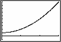
This is the graph of y = x² + 1, the solution to the initial value problem.

20.2.3 Use EULERG to graph the solution to the initial value problem with y(1) = 1 in a
[0, 10, 1] x [-1, 10, 5] window. Use 0.01 for the STEP SIZE.

Click here for the answer.

y' as a Function of y

EULERG can also be used to graph solutions to differential equations that depend on both x and y.

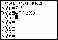
Graph the solution to the initial-value problem y' = 2y with y(0) = 1 using the EULERG program.

• Enter Y1 = 2Y.
• Enter a [0, 2, 1] x [-1, 20, 5] viewing window.
• Run program EULERG.
• Enter 0 for the initial value of X.
• Enter 1 for the initial value of Y.
• Enter 0.01 for the STEP SIZE.

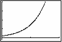
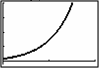
This is a graphical solution to the initial value problem. The analytical solution is y = e^2x. Graph y = e^2x to compare with the solution given by EULERG.

• Enter Y₂ = e^(2X). The exponential function is above the key.
• Change the viewing style of Y2 to thick.
• Y₁ should still be unselected.

• Press . You should see y = e^2x graphed over the curve drawn by EULERG.

Note that the analytical solution to y' = 2y was not found by evaluating an indefinite integral. Several types of differential equations require other techniques to produce solutions and many differential equations do not have analytically determined solutions at all.

EULERG Program EULERG uses "Euler's method" and is only an approximation. It can be very inaccurate if the step sizes are too large, OR if the interval is too large, OR if you get too near a vertical tangent line.