3D Graphing
The 3D Graphing view lets you view and explore three-dimensional graphs of:
|
•
|
3D functions of the form z(x,y) |
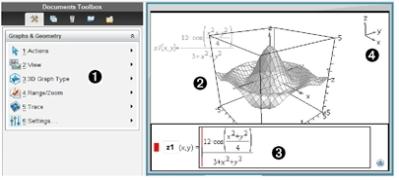
While you are in the 3D Graphing view, you can define, rotate, resize, and trace 3D graphs. You can set the colors and other visual attributes of a selected graph, and you can customize the 3D viewing environment.
|
À
|
3D Graphing menu. This menu is specific to 3D Graphing and is accessible from the Graphs & Geometry menu.
|
|
Á
|
Sample 3D graph. Each 3D graphing page can show multiple graphs.
|
|
Â
|
Entry line with expression that defines the graph
|
|
Ã
|
Legend displaying orientation of the axes
|
Operators and Functions Supported
You can use any of the following items in an expression for 3D graphing:
+ N Q P ^
explnlog
sqrtabsceilingfloorintsignroot
realimagconj
sincostanseccsccot
arcsinarccosarctanarcsecarccscarccot
sinhcoshtanhsechcschcoth
arcsinharccosharctanharcsecharccscharccoth
Graphing 3D Functions
|
1.
|
From the menu, click . |
|
2.
|
From the menu, click . |
The entry line appears.

|
3.
|
Type the expression that defines the graph. |
|
4.
|
Press · to draw the graph and hide the entry line. You can show or hide the entry line anytime by pressing /. |
Graphing 3D Parametric Equations
|
1.
|
From the menu, click . |
|
2.
|
From the menu, click . |
The entry line appears.
|
3.
|
Type the equations that define the graph. |
|
4.
|
(Optional) Click the Edit Parameters button  to set the graphing parameters tmin, tmax, umin, and umax. to set the graphing parameters tmin, tmax, umin, and umax. |
|
5.
|
Press · to draw the graph and hide the entry line. You can show or hide the entry line anytime by pressing /. |
Displaying the Context Menu of a 3D Graph
Some 3D graphing features are accessible only through context menus.
|
1.
|
If necessary, press d to return to the Pointer tool. |
|
2.
|
Point to the graph to select it. |
The selected graph is displayed in gray.
|
3.
|
Display the graph’s context menu. |
|
-
|
Mac®: Hold “ and click. |
Editing a 3D Graph
|
1.
|
Display the graph’s context menu, and then click . |
—or—
Press / to show the entry line, and use the up/down arrow keys to display the expression.
|
2.
|
Modify the existing expression, or type a new expression in the entry line. |
Changing the Color or Appearance of a 3D Graph
To Set Wire and Surface Color:
|
1.
|
Display the graph’s context menu, click , and then click or . |
|
2.
|
Click a color swatch to apply it. |
To Set Custom Plot Colors:
Custom plot colors can make it easier to see the shape characteristics of the graph. You can assign different colors to its top and bottom surfaces or choose to have the graph colored automatically, based on height or steepness. You can also set the wire color.
|
1.
|
Display the graph’s context menu, and then click > . |
|
2.
|
Select one of the three Surface color options: , , or . |
|
-
|
If you choose Top/bottom color, click the color swatches to select colors for the top and bottom surfaces. |
|
-
|
If you choose to vary color by height or steepness, colors are determined automatically. |
|
3.
|
To set the Wire color, click the color swatch and select a color. |
To Set Other Attributes of a Graph:
|
1.
|
Display the graph’s context menu, and then click . You can set the following attributes for the selected graph. |
|
-
|
format: surface+wire, surface only, or wire only |
|
-
|
x resolution (enter a value in range 2-200*, default=) |
|
-
|
y resolution (enter a value in range 2-200*, default=) |
|
-
|
transparency (enter a value in range 0-100, default=) |
|
-
|
shading (controls highlights, enter a value in range 0-100, default=) |
* Handhelds are limited to a maximum display resolution of 21, regardless of the value entered.
|
2.
|
Set the attributes as you like. For more information, see Changing an Attribute of an Object. |
|
3.
|
Press · to accept the changes. |
If a Graph is Difficult to Select
|
1.
|
From the menu, click the graph’s type (either or ). |
The entry line appears.
|
2.
|
Use the up/down arrow keys to select the graph. |
|
3.
|
Display the graph’s context menu. |
|
-
|
Mac®: Hold “ and click. |
|
4.
|
Click the menu item that you want to change. |
Showing and Hiding 3D Graphs
To Hide a 3D Graph:
|
¢
|
Display the graph’s context menu, and then click . |
To Show a Hidden 3D Graph:
|
1.
|
From the menu, click . |
The Hide/Show icon  appears and all hidden graphs show in gray.
|
2.
|
Click a graph to change its hide/show state. |
|
3.
|
To return to the Pointer tool, press d. |
Customizing the 3D Viewing Environment
To Set the Background Color:
|
¢
|
Display the context menu for the work area, and then click . |
To Show or Hide Specific View Elements:
|
¢
|
From the menu, click the item to show or hide. You can choose items such as the 3D box, axes, box end values, and legend. |
To Set the Visual Attributes of the Box and Axes:
|
1.
|
Display the context menu for the box, and then click . You can set the following attributes. |
|
-
|
Show or hide tic labels |
|
-
|
Show or hide end values |
|
-
|
Show or hide arrows on axes |
|
-
|
Show 3D or 2D arrow heads |
|
2.
|
Set the attributes as you like. For more information, see Changing an Attribute of an Object. |
|
3.
|
Press · to accept the changes. |
To Shrink or Magnify the 3D View:
|
¢
|
From the menu, click or . |
To Change the 3D Aspect Ratio:
|
1.
|
From the menu, click . |
|
2.
|
Enter values for the x, y, and z axes. The default value for each axis is . |
To Change the Range Settings
|
¢
|
On the menu, click . You can set the following parameters. |
|
-
|
XMin (default=)
XMax (default=)
XScale (default=) You can enter a numeric value. |
|
-
|
YMin (default=)
YMax (default=)
YScale (default=) You can enter a numeric value. |
|
-
|
ZMin (default=)
ZMax (default=)
ZScale (default=) You can enter a numeric value. |
|
-
|
eye q¡ (default=)
eye f¡ (default=)
eye distance (default=) |
Rotating the 3D View
To Rotate Manually:
|
1.
|
Press to activate the Rotation tool (required only for the TI‑Nspire™ handheld with Clickpad). |
|
2.
|
Press any of the four arrow keys to rotate the graph. |
To Rotate Automatically:
Auto rotation is equivalent to holding down the right arrow key.
|
1.
|
From the menu, click . |
The Auto Rotation icon  appears, and the graph rotates.
|
2.
|
(Optional) Use the up and down arrow keys to explore the rotating graph. |
|
3.
|
To stop the rotation and return to the Pointer tool, press d. |
To View from Specific Orientations:
|
1.
|
If necessary, press d to return to the Pointer tool. |
|
2.
|
Use letter keys to select the orientation: |
|
-
|
Press , , or to view along the z, y, or x axis. |
|
-
|
Press letter to view from the default orientation. |
Tracing in the 3D View
To Start Tracing:
|
1.
|
From the menu, click . |
The z Trace icon  and the trace plane appear, along with a text line showing the current "z=" trace value.
|
2.
|
To move the trace, hold down and press the up or down arrow key. |
The "z=" text is updated as you move.
|
3.
|
(Optional) Use the four arrow keys to rotate the view and see how the trace plane and the graph intersect. |
|
4.
|
To stop tracing and return to the Pointer tool, press d. |
To Change the Trace Settings:
|
1.
|
From the menu, click . |
The 3D Trace Setup dialog box opens.
|
2.
|
Enter or select the settings, and click to apply them. |
|
3.
|
If you are not already tracing, your new settings take effect the next time you trace. |
Animating a 3D Graph with a Slider
The following steps illustrate an example of an animated 3D graph.
|
1.
|
Insert a new problem and select the 3D Graphing view. |
|
2.
|
From the menu, click , click to position it, and type time as the variable name. |
|
3.
|
Display the slider’s context menu, click , and enter the following values. |
Value:
Minimum:
Maximum:
Step Size:
|
4.
|
In the entry line, define the function shown here: |
|
5.
|
Drag the slider thumb to see the effect of varying time. |
|
6.
|
Add visual interest. For example, try: |
|
-
|
Hiding the box, axes, and legend. |
|
-
|
Setting the graph’s format attribute to show the surface only. |
|
-
|
Changing the graph’s transparency and shading attributes. |
|
-
|
Changing the background color and graph fill color. |
|
7.
|
To animate the graph, display the slider’s context menu, and click . (To stop, click from the context menu.) |
You can combine manual or auto rotation with the slider animation. Experiment with the x and y resolution to balance curve definition against animation smoothness.