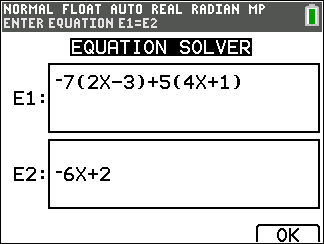
| 1. | Enter an equation as expression 1=expression 2 (E1=E2). |
You may enter more than one variable, but you will have to select one variable to solve. The other variables used will take on the value stored in the calculator.
| 2. | Press OK. |
| 3. | Place the cursor on the variable to solve. For this example, the variable is X. |
The current value of X stored in the calculator is displayed (X=0).
You should enter a value close to your estimate of the solution. If needed, you can look at the intersection of the graph of both sides of your equation or use the table of values to know more about your problem. Here, X=0 is a reasonable starting point for the calculator computation.
Bound – {-1E99, 1E99} represents the calculator version of the Real Number line:
{-1x1099, 1x1099}. You can change this interval if you know about where the solution lies given your study of a graph or table. For most textbook problems, you probably will not have to change this line.
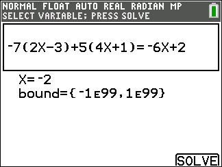
| 4. | Press the [SOLVE] (s) shortcut key. |
| 5. | Check your solution. The calculator checks the solution it generated. |
|
Always read the context help line for tips. |
|
|
The solution will be marked with a small square. |
|
|
(Advanced) Bounds gives the interval where the solution is found. Here, {-1E99, 1E99} is {-1x1099, 1x1099} which has the calculator looking for the solution within a very large interval of numbers. You can adjust this interval if you do not get all the solutions to your equation by limiting the values to a smaller interval. Here, there is only one solution, |
|
|
E1-E2=0 (expression 1 = expression 2) is finding the difference of the left hand side of your equation, E1 with X=-2 and the right hand side of your equation, E2 with X=-2. The difference is zero. The equation balances. X=-2 is the solution. (Advanced: When E1=E2 is not zero, but is a small value, the calculator algorithm likely gave a result close to the exact answer but within some tolerance of the calculator arithmetic.) |
|