You can perform statistical calculations to analyse data. The following example fits a y=mx+b linear regression model to the two lists in columns A and B.

1.

From the Statistics menu, select Stat Calculation > LinearRegression (mx+b) to choose the regression model.

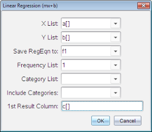
The Linear Regression (mx+b) dialogue box opens.

2.

Type a[] as the column for the X List.

3.

Type b[] as the column for the Y List.

4.

To store the regression equation in a specified variable, replace Save RegEqn To with the name of the variable.

5.

Type c[] as the column for the 1st Result.

6.

Click OK.

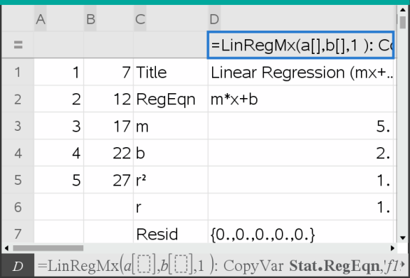
Lists & Spreadsheet inserts two columns: one containing the names of the results, and one containing the corresponding values.

Note: The results are linked to the source data. For example, if you change a value in column A, the regression equation is updated automatically.

 

Lists & Spreadsheet stores statistical results using a variable-group name with the format stat.nnn, where nnn is the result name (for example, stat.RegEqn and stat.Resid). The use of standard names for variables makes it easier to identify and use the statistical variables later. If you want to use a custom variable group instead of the standard name, you can edit the formula in the column formula cell.

You could use the following formula to store the results in the variable group MystatsB.

=LinRegMx(a[],b[],1 ): CopyVar Stat., MystatsB.

Later, you could view the results by entering the following expression in the Calculator application or in another column of the Lists & Spreadsheet application:

MystatsB.results

 

The Stat Calculations menu lets you select from the calculations described below. For more information, see the TI-Nspire™ Reference Guide.

One-Variable Statistics (OneVar)

Analyses data with one measured variable. You can specify an optional frequency list. The statistical data returned using this analysis technique are:

•

Sample mean, x

•

Sum of the data, Gx

•

Sum of the squared data, Gx2

•

Sample standard deviation, sx

•

Population standard deviation, sx

•

Sample size, n

•

X-min

•

First quartile, Q1

•

Median

•

Third quartile, Q3

•

X-max

•

Sum of squared deviations, SSx = G(x Nx)2

Two-Variable Statistics (TwoVar)

Analyses paired data. List 1 is the independent variable. List 2 is the dependent variable. You can specify an optional frequency list. The statistical data returned using this analysis technique are:

For each list:

•

Sample mean, x or y

•

Sum of the data, Gx or Gy

•

Sum of the squared data, Gx2 or Gy2

•

Sample standard deviation, sx = sn-1x or sy = sn-1y

•

Population standard deviation, sx = snx or sy = sny

•

X-min or Y-min

•

First quartile, Q1X or Q1Y

•

Median

•

Third quartile, Q3X or Q3Y

•

X-max or Y-max

•

Sum of squared deviations, SSx = G(x Nx)2 or SSy = G(y Ny)2

Additional data:

•

Sample size for each data set, n

•

Gxy

•

Correlation coefficient, R.

Linear Regression (mx+b) (LinRegMx)

Fits the model equation y=ax+b to the data using a least-squares fit. It displays values for m (slope) and b (y-intercept).

Linear Regression (a+bx) (LinRegBx)

Fits the model equation y=a+bx to the data using a least-squares fit. It displays values for a (y-intercept), b (slope), r2, and r.

Median-Median Line (MedMed)

Fits the model equation y=mx+b to the data using the median-median line (resistant line) technique, calculating the summary points x1, y1, x2, y2, x3 and y3. Median-Median Line displays values for m (slope) and b (y-intercept).

Quadratic Regression (QuadReg)

Fits the second-degree polynomial y=ax2+bx+c to the data. It displays values for a, b, c, and R2. For three data points, the equation is a polynomial fit; for four or more, it is a polynomial regression. At least three data points are required.

Cubic Regression (CubicReg)

Fits the third-degree polynomial y=ax3+bx2+cx+d to the data. It displays values for a, b, c, d, and R2. For four points, the equation is a polynomial fit; for five or more, it is a polynomial regression. At least four points are required.

Quartic Regression (QuartReg)

Fits the fourth-degree polynomial y=ax4+bx3+cx2+dx+e to the data. It displays values for a, b, c, d, e and R2. For five points, the equation is a polynomial fit; for six or more, it is a polynomial regression. At least five points are required.

Power Regression (PowerReg)

Fits the model equation y=axb to the data using a least-squares fit on transformed values ln(x) and ln(y). It displays values for a, b, r2 and r.

Exponential Regression (ExpReg)

Fits the model equation y=abx to the data using a least-squares fit on transformed values x and ln(y). It displays values for a, b, r2 and r.

Logarithmic Regression (LogReg)

Fits the model equation y=a+b ln(x) to the data using a least-squares fit on transformed values ln(x) and y. It displays values for a, b, r2 and r.

Sinusoidal Regression (SinReg)

Fits the model equation y=a sin(bx+c)+d to the data using an iterative least-squares fit. It displays values for a, b, c and d. At least four data points are required. At least two data points per cycle are required to avoid aliased frequency estimates.

Note: The output of SinReg is always in radians, regardless of the Radian/Degree mode setting.

Logistic Regression (d=0) (Logistic)

Fits the model equation y=c/(1+a*e-bx) to the data using an iterative least-squares fit. It displays values for a, b and c.

Logistic Regression (dƒ0) (LogisticD)

Fits the model equation y=c(1+a*e(-bx))+d to the data using an iterative least-squares fit. It displays values for a, b, c and d.

Multiple Linear Regression (MultReg)

Calculates multiple linear regression of list Y on lists X1, X2, …, X10.