In the Vernier DataQuest™ application, use Graph View to analyze data. Start by setting up graphs, and then use analysis tools such as integral, statistics, and curve fit to investigate the mathematical nature of the data.
Important: The Graph menu and Analyze menu items are only available when working in Graph View.
Use Integral to determine the area under a data plot. You can find the area under all of the data or a selected region of the data.
To find the area under a data plot:
| 1. | Leave the graph unselected to examine all the data, or select a range to examine a specific area. |
| 2. | Click Analyze > Integral. |
| 3. | Select the plotted column name if you have more than a single column. |
The data plot area is displayed in the View Details area.
Tangent displays a measure of the rate at which the data is changing at the point you are examining. The value is labeled “Slope.”
To find the slope:
| 1. | Click Analyze > Tangent. |
A check mark appears in the menu next to the option.
| 2. | Click the graph. |
The examine indicator is drawn to the nearest data point.
The values of the plotted data are shown in the View details area and the All Details for Graph dialog box.
You can move the examine line by dragging, clicking another point, or using the arrow keys.
Use Interpolate to estimate the value between two data points and to determine the value of a Curve Fit between and beyond these data points.
The examine line moves from data point to data point. When Interpolate is on, the examine line moves between and beyond data points.
To use Interpolate:
| 1. | Click Analyze > Interpolate. |
A check mark appears in the menu next to the option.
| 2. | Click the graph. |
The examine indicator is drawn to the nearest data point.
The values of the plotted data are shown in the View Details area.
You can shift the examine line by moving the cursor with the arrow keys or by clicking on another data point.
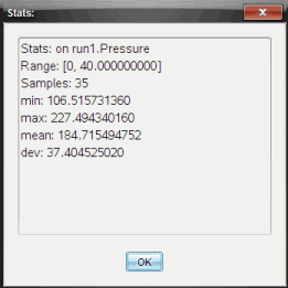
You can generate statistics (minimum, maximum, mean, standard deviation, and number of samples) for all the collected data or for a selected region. You can also generate a curve fit based on one of several standard models or on a model that you define.
| 1. | Leave the graph unselected to examine all the data, or select a range to examine a specific area. |
| 2. | Click Analyze > Statistics. |
| 3. | Select the plotted column name if you have more than a single column. For example, run1.Pressure. |
The Stats dialog box opens.

| 4. | Review the data. |
| 5. | Click OK. |
For information on clearing the Statistics analysis, see Removing Analysis Options.
Use Curve Fit to find the best curve fit to match the data. Select all of the data or a selected region of data. The curve is drawn on the graph.
| 1. | Leave the graph unselected to examine all the data, or select a range to examine a specific area. |
| 2. | Click Analyze > Curve Fit. |
| 3. | Select a curve fit option. |
|
Calculated in the form: |
|
|
Linear |
y = m*x + b |
|
Quadratic |
y = a*x^2 + b*x + c |
|
Cubic |
y = a*x^3 + b*x^2 + c*x + d |
|
Quartic |
y = a*x^4 + b*x^3 + c*x^2 + d*x + e |
|
Power (ax^b) |
y = a*x^b |
|
Exponential (ab^x) |
y = a*b^x |
|
Logarithmic |
y = a + b*ln(x) |
|
Sinusoidal |
y = a*sin(b*x + c) + d |
|
Logistic (d |
y = c/(1 + a*e^(-bx)) + d |
|
Natural Exponential |
y = a*e^(-c*x) |
|
Proportional |
y = a*x |
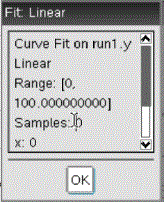
The Fit Linear dialog box opens.

| 4. | Click OK. |
| 5. | Review the data. |
For information on clearing the Curve Fit analysis, see Removing Analysis Options.
This option provides a manual method for plotting a function to fit data. Use one of the predefined models or enter your own.
You can also set the spin increment to use in the View Details dialog box. Spin increment is the value by which the coefficient changes when you click the spin buttons in the View Details dialog box.
For example, if you set m1=1 as the spin increment, when you click the up spin button the value changes to 1.1, 1.2, 1.3 and so on. If you click the down spin button, the value changes to 0.9, 0.8, 0.7, and so on.
| 1. | Click Analyze > Model. |
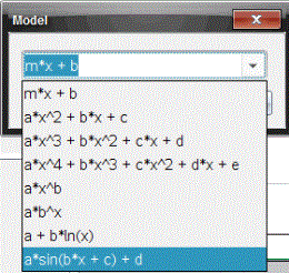
The Model dialog box opens.

| 2. | Type your own function. |
—or—
Click to select a value from the drop-down list.
| 3. | Click OK. |
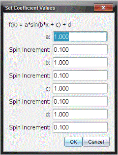
The Set Coefficient Values dialog box opens.

| 4. | Type the value for the variables. |
| 5. | Type the change in value in the Spin Increment fields. |
| 6. | Click OK. |
Note: These values are the initial values. You can also adjust these values in the View Details area.
The model is shown on the graph with adjustment options in the View Details area and in the All Details for Graph dialog box.
| 7. | (Optional) Adjust the window setting for minimum and maximum axis values. For more information, see Setting the Axis for One Graph. |
For information on clearing the Model analysis, see Removing Analysis Options.
| 8. | Click  to make any desired adjustments to the coefficients. to make any desired adjustments to the coefficients. |
—or—
Click the value in the View Details area.
This graphic is an example of a model with adjusted values.
| 1. | Click Analyze > Remove. |
| 2. | Select the data display you want to remove. |
The display you selected is removed from the graph and the View Details area.
 Finding the Area Under a Data Plot
 0)
0)