Utilisez les exemples de scripts suivants pour vous familiariser avec les méthodes décrites à la section Référence. Par ailleurs, ces exemples comprennent plusieurs scripts
TI-Innovator™ Hub et TI-Innovator Rover™ qui faciliteront votre prise en main du langage TI-Python.
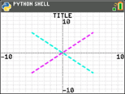
import ti_plotlib as plt
plt.cls()
plt.window(-10,10,-10,10)
plt.axes("on")
plt.grid(1,1,"dot")
plt.title("TITLE")
plt.pen("medium","solid")
plt.color(28,242,221)
plt.pen("medium","dash")
plt.line(-5,5,5,-5,"")
plt.color(224,54,243)
plt.line(-5,-5,5,5,"")
plt.show_plot()
Appuyez sur ‘ pour afficher l'invite du Shell.
Configurez une équation de régression avant d'exécuter le script Python dans l'application Python. Par exemple, vous pourriez tout d'abord saisir deux listes dans le système d'exploitation (OS) CE. Puis, par exemple, calculez [stat] CALC 4:LinReg(ax+b) pour vos listes. Cela permet de stocker l'équation de régression dans RegEQ dans l'OS. Voici un script destiné à rappeler RegEQ dans l'expérience Python.
# Exemple d'utilisation de recall_RegEQ()
from ti_system import *
reg=recall_RegEQ()
print(reg)
x=float(input("Input x = "))
print("RegEQ(x) = ",eval(reg))
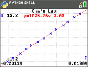
import ti_plotlib as plt
# intensité du courant
I = [0.0, 0.9, 2.1, 3.1, 3.9, 5.0, 6.0, 7.1, 8.0, 9.2, 9.9, 11.0,11.9]
# tension
for n in range (len(I)):
I[n] /= 1000
# tension
U = [0, 1, 2, 3.2, 4, 4.9, 5.8, 7, 8.1, 9.1, 10, 11.2, 12]
plt.cls()
plt.auto_window(I,U)
plt.pen("thin","solid")
plt.axes("on")
plt.grid(.002,2,"dot")
plt.title("Loi d'Ohm")
plt.color (0,0,255)
plt.labels("I","U",11,2)
plt.scatter(I,U,"x")
plt.color (255,0,0)
plt.pen("thin","dash")
plt.lin_reg(I,U,"center",2)
plt.show_plot()
plt.cls()
a=plt.a
b=plt.b
print ("a =",round(plt.a,2))
print ("b =",round(plt.b,2))
Appuyez sur ‘ pour afficher l'invite du Shell.
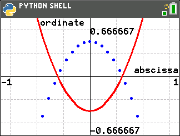
import ti_plotlib as plt
#Après avoir exécuté le script, appuyez sur [annul] pour effacer le tracé et revenir au Shell.
def f(x):
••return 3*x**2-.4
def g(x):
••return -f(x)
def plot(res,xmin,xmax):
••#configurer la zone de tracé
••plt.window(xmin,xmax,xmin/1.5,xmax/1.5)
••plt.cls()
••gscale=5
••plt.grid((plt.xmax-plt.xmin)/gscale*(3/4),(plt.ymax-plt.ymin)/gscale,"dash")
••plt.pen("thin","solid")
••plt.color(0,0,0)
••plt.axes("on")
••plt.labels("abscisse"," ordonnee",6,1)
••plt.pen("medium","solid")
# tracer f(x) et g(x)
dX=(plt.xmax -plt.xmin)/res
x=plt.xmin
x0=x
••for i in range(res):
••••plt.color(255,0,0)
••••plt.line(x0,f(x0),x,f(x),"")
••••plt.color(0,0,255)
••••plt.plot(x,g(x),"o")
••••x0=x
••••x+=dX
••plt.show_plot()
#plot (résolution,xmin,xmax)
plot(30,-1,1)
# Créer un graphique avec les paramètres (résolution,xmin,xmax)
# Après avoir effacé le premier graphique, appuyer sur la touche [var]. La fonction plot() permet de modifier les paramètres d’affichage (résolution,xmin,xmax).
Appuyez sur ‘ pour afficher l'invite du Shell.
Voir : [Fns…]>Modul: module ti_hub
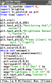
from ti_system import *
import brightns
import ti_plotlib as plt
from time import *
plt.cls()
plt.color(0,0,255)
plt.text_at(2,"Monitoring Hub","center")
plt.text_at(3,"Brightness Sensor","center")
plt.color(255,0,0)
plt.text_at(12,"Press [annul] to quit ","right")
t0=monotonic()
plt.color(0,0,0)
while not escape():
••I=brightns.measurement()
••I=round(I,1)
••tf=monotonic()
••plt.color(0,0,0)
••tm=round(tf-t0,1)
••msg="Time = %.1f sec" % tm
••plt.text_at(6,msg,"center")
••msg="Brightness = %.1f %%" %I
••plt.text_at(7,msg,"center")
••sleep(1)
Voir : [Fns…]>Modul module ti_rover
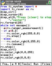
from ti_system import *
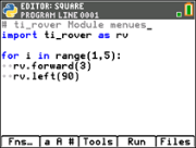
import ti_rover as rv
disp_clr()
disp_cursor(0)
disp_at(6,"Press [annul] to stop","center")
rv.forward(20)
while not escape():
••a=rv.ranger_measurement()
••if a<0.2:
••••rv.color_rgb(255,0,0)
••••rv.stop()
••else:
••••rv.color_rgb(0,255,0)
••••rv.resume()
rv.stop()
disp_clr()
rv.color_rgb(0,0,255)
sleep(1)
rv.color_rgb(0,0,0)
Voir : [Fns…]>Modul: module ti_hub
Voir : [Fns…]>Modul module ti_rover
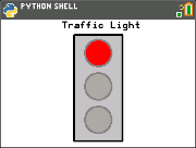
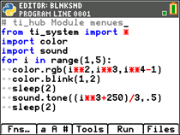
from ti_draw import *
from ti_image import *
from time import *
clear()
# Pixel screen upper left (0,0) to (319,209)
draw_text(100,20,"Traffic Light")
set_pen("medium","solid")
draw_rect(120,25,80,175)
set_color(192,192,192)
fill_rect(120,25,80,175)
set_color(128,128,128)
draw_circle(160,55,22)
draw_circle(160,110,22)
draw_circle(160,165,22)
def off(x,y):
••set_color(169,169,169)
••fill_circle(x,y,22)
••set_color(128,128,128)
••draw_circle(x,y,22)
for i in (1,20,1):
# Green
••set_color(51,165,50)
••fill_circle(160,165,22)
••sleep(3)
••off(160,165)
# Yellow
••set_color(247,239,10)
••fill_circle(160,110,22)
••sleep(2)
••off(160,110)
# Red
••set_color(255,0,0)
••fill_circle(160,55,22)
••sleep(3)
••off(160,55)
••show_draw()