Calculating Amortization

Calculating an Amortization Schedule

Use the amortization functions (menu items 9, 0, and A) to calculate balance, sum of principal, and sum of interest for an amortization schedule.

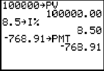
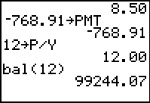
bal(

bal( computes the balance for an amortization schedule using stored values for æ, PV, and PMT. npmt is the number of the payment at which you want to calculate a balance. It must be a positive integer < 10,000. roundvalue specifies the internal precision the calculator uses to calculate the balance; if you do not specify roundvalue, then the graphing calculator uses the current Float/Fix decimal-mode setting.

bal(npmt[,roundvalue])

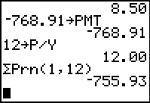
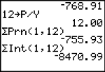
GPrn(, GInt(

GPrn( computes the sum of the principal during a specified period for an amortization schedule using stored values for ¾æ, PV, and PMT. pmt1 is the starting payment. pmt2 is the ending payment in the range. pmt1 and pmt2 must be positive integers < 10,000. roundvalue specifies the internal precision the calculator uses to calculate the principal; if you do not specify roundvalue, the graphing calculator uses the current Float/Fix decimal-mode setting.

Note: You must enter values for æ, PV, and PMT before computing the principal.

GPrn(pmt1,pmt2[,roundvalue])

GInt( computes the sum of the interest during a specified period for an amortization schedule using stored values for ¾æ, PV, and PMT. pmt1 is the starting payment. pmt2 is the ending payment in the range. pmt1 and pmt2 must be positive integers < 10,000. roundvalue specifies the internal precision the calculator uses to calculate the interest; if you do not specify roundvalue, the TI‑84 Plus C uses the current Float/Fix decimal-mode setting.

GInt(pmt1,pmt2[,roundvalue])

 

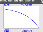
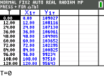
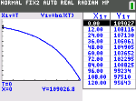
Amortization Example: Calculating an Outstanding Loan Balance

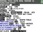
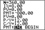
You want to buy a home with a 30-year mortgage at 8 percent APR. Monthly payments are 800. Calculate the outstanding loan balance after each payment and display the results in a graph and in the table.

1. Press z. Press † ~ ~ ~ [enter] to set the fixed‑decimal mode setting to 2. Press † † ~ [enter] to select Par graphing mode.
2. Press Π[enter] [enter] to display the TVM Solver.
3. Press 360 to enter number of payments. Press † 8 to enter the interest rate. Press † † Ì 800 to enter the payment amount. Press †0 to enter the future value of the mortgage. Press † 12 to enter the payments per year, which also sets the compounding periods per year to 12. Press † † [enter] to select PMT:END.
4. Move the cursor to the PV prompt and then press ƒ \ to solve for the present value.
5. Press o to display the parametric Y= editor. Turn off all stat plots. Press „ to define X1T as T. Press † Œ [enter] 9 „ ¤ to define Y1T as bal(T).
6. Press p to display the window variables. Enter the values below. Tmin=0 Xmin=0 Ymin=0 Tmax=360Xmax=360Ymax=125000 Tstep=12 Xscl=50 Yscl=10000
7. Press r to draw the graph and activate the trace cursor. Press ~ and | to explore the graph of the outstanding balance over time. Press a number and then press [enter] to view the balance at a specific time T.
8. Press y - and enter the values below. TblStart=0 @Tbl=12
9. Press y 0 to display the table of outstanding balances (Y1T).
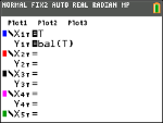
10. Press z and select Graph‑Table split-screen mode, so that the graph and table are displayed simultaneously. Press r to display X1T (time) and Y1T (balance) in the table.