Motion along a straight line was illustrated in Lesson 12.1. This lesson will explore harmonic motion, that is, motion that oscillates.

Simple harmonic motion is motion that can be modeled by either of the following functions, where t is time:

f(t) = a sin (bt + c) + d             or              g(t) = a cos(bt + c) + d

Stating the Problem

A particle moves along the vertical line x = 1 according to the equation . Model the motion of the particle from t = 0 to t = 5 seconds using parametric equations.

Modeling the Particle's Motion

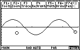
The graph of the following parametric equations illustrates when the particle is moving up, when it is moving down, and when it is at rest.

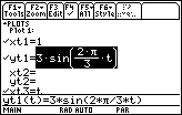
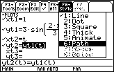
• Set xt1 = 1
  This represents the vertical line on which the particle moves.
• Set yt1 = 3*sin(2* /3*t)
  This represents the motion of the particle along its path.

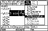
• Set the Graph Style of yt1 to Animate

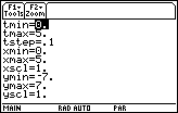
• Enter the Viewing Window values shown below

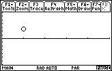
• Display the graph

You should see the ball rise and fall along the vertical line x = 1.

• Display the Window Editor by pressing
• Change the value of tstep to 0.05
• Display the graph again

12.2.1 What is the effect of this change on the graph?
Click here for the answer.

Another Model

Add the following pair of equations to the Y= Editor to produce another model for the particle motion.

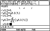
• Set xt2 = t
• Set yt2 = yt1(t)
• Select "Path" for the Graph Style for this pair of equations

• Make sure the Graph Order in the 9:Format dialog box is still Simultaneous
• Display the graphs.
  Unfortunately, only the new pair appears to be graphed because no settings were changed for the first pair.
• Press to regraph.

12.2.2 Use the Trace feature on the second graph to determine when the particle is moving upward.
Click here for the answer.

12.2.3 When is the particle moving downward?
Click here for the answer.

12.2.4 When is the particle at rest?
Click here for the answer.

Graphing the Derivative

Add the following equations to the Y= Editor to see the derivative (velocity) of the particle.

• Set xt3 = t
• Set yt3 = d(yt1(t),t)

• Display the graphs

12.2.5 Use Trace on the velocity curve to find the first time when the particle is at rest.
Click here for the answer.

12.2.6 What feature of the derivative tells you when the particle is moving up or down?
Click here for the answer.