In this lesson you will calculate and compare average velocities of a falling object over several different time intervals and then graphically illustrate these velocities.

The following experiment was conducted to illustrate the concept of average velocity. The data from the experiment will be used to create a scatter plot and to find average velocities.

An Experiment: Dropping a Book

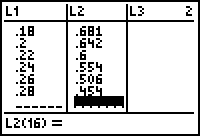
A book was dropped from a height of 0.865 meters and its height above ground was monitored with a Texas Instruments Calculator-Based Laboratory™ (CBL™). The following table contains data of the book's height in meters versus time in seconds.

Time	0.00	0.02	0.04	0.06	0.08	0.10	0.12
Height	0.865	0.858	0.848	0.836	0.819	0.799	0.775

Time	0.14	0.16	0.18	0.20	0.22	0.24	0.26	0.28
Height	0.748	0.716	0.681	0.642	0.600	0.554	0.506	0.454

Entering the Data

To create a scatter plot of the data and explore average velocities, the data must be entered into the Stat List editor.

• Open the editor by pressing .
• Clear the contents of each list by placing the cursor on top of the list heading and pressing .
• Enter the times in L1 and the heights in L2.

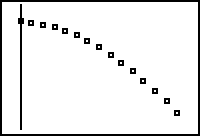
Making a Scatter Plot of Height (y) versus Time (x)

• Open the Plot Setup screen and select Plot1 by pressing [STATPLOT] .
• Enter the values shown in the following screen.

• Display the scatter plot in a Zoom Statistics window by pressing and selecting 9:ZoomStat.
  Zoom Statistics defines a window that displays all statistical data points.

Average Velocity

Average velocity is defined to be the change in position divided by elapsed time.

If h₁ is the height at time t₁ and h₂ is the height at time t₂ :

h₂ - h₁ represents change in position,

t₂ - t₁ represents elapsed time, and

represents average velocity.

Finding the Average Velocity

Find the average velocity of the book from t = 0 to t = 0.28 by using the points (0, 0.865) and (0.28, 0.454).

• On the Home screen enter the command (0.454 - 0.865) / (0.28 - 0).

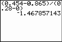
The average velocity over the interval from t = 0 to t = 0.28 was approximately -1.468 m/s. The negative sign means that the object is moving downward.

Finding the Average Velocity over Subintervals

9.1.1 Approximate the average velocity

1. from t = 0 to t = 0.16 by using the points (0, 0.865) and (0.16, 0.716).
2. from t = 0.16 to t = 0.28 by using the points (0.16, 0.716) and (0.28, 0.454).

Click here for the answer.

9.1.2 The second average velocity has a larger magnitude than the first. Describe what this tells you about the falling object. Click here for the answer.

Slope as Average Velocity

Compare the following two expressions.

1. The slope of a line through the points (x₁, y₁) and (x₂, y₂) is given by .
2. The average velocity between the points (t₁, h₁) and (t₂, h₂) is given by .

Because slope and average velocity are computed the same way, the average velocity from t = 0 to t = 0.28 can be represented as the slope of the line through the corresponding points on the scatter plot.

Drawing Line Segments

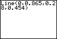
To illustrate the average velocity between two points, you can graph a line segment through the points with the Line command, which is found in the Draw menu.

Draw the line segment through the points that represent t = 0 and t = 0.28.

• Go to the Home screen and open the Draw menu by pressing [DRAW].
• Paste "Line(" to the Home screen by selecting 2:Line(.

The syntax for the Line command is Line(x1,y1,x2,y2) and the two points are (0, 0.865) and (0.28, 0.454).

• Complete the command Line(0,0.865,0.28,0.454).

• Press to execute the command.

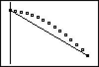
The slope of this line segment is the average velocity for the entire time interval given in the table.

The Line Command The Line command can be used from the Home screen by entering Line(x1,y1,x2,y2), as described above, or from the Graph screen. To draw a line when a graph is displayed: Open the DRAW menu and select 2:Line(. Place the cursor on either end of the desired line segment and press . Use the arrow keys to move to the other end of the desired line segment and press .

Illustrating Average Velocities on Subintervals

The average velocity of the book during the subinterval from t = 0 to t = 0.16 can be illustrated by drawing the line segment that contains the points (0, 0.865) and (0.16, 0.716).

• Return to the Home screen by pressing [QUIT].
• Enter the command Line(0,0.865,0.16,0.716).

 

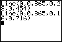
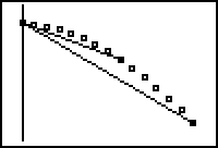
Illustrate the average velocity between t = 0.16 and t = 0.28 by drawing the line segment between the points (0.16, 0.716) and (0.28, 0.454).

• Return to the Home screen by pressing [QUIT].
• Enter the command Line(0.16,0.716,0.28,0.454).

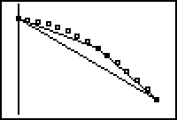
The slope of each line segment is the average velocity over the corresponding time interval.

Clearing the Line Segments

• In preparation for Lesson 9.2, display the scatter plot without the lines by pressing [DRAW] and selecting 1:ClrDraw.